The nature of variability (variations, changeability) is the basis of statistical thinking that is different from thinking in terms of tolerances
This section of the site is dedicated to explaining the need to understand the nature of variability to manage any systems (social, business, industrial and technical), because we live in a world filled with variability. The importance of understanding the laws of variability for improving quality and increasing the efficiency of production and services cannot be overestimated; this knowledge is as important as understanding the laws of aerodynamics if you are designing aircraft.
Material prepared by: Scientific Director of the AQT Center Sergey P. Grigoryev .
Free access to articles does not in any way diminish the value of the materials contained in them.
Variability – variability, diversity, scatter or measure of deviation from the “optimum”. The change itself is called a variation or variant.
“The fundamental problem in management, leadership and production, as my friend Lloyd Nelson has formulated it and as we have emphasized many times, is a failure to understand and interpret the nature of variation.
Efforts and practices to improve quality and productivity in most companies and government agencies are fragmented, with neither overall competent leadership nor a cohesive system of continuous improvement.
Everyone, regardless of their position, needs training and development. In an atmosphere of fragmented efforts, people move each in their own direction, unable to bring greater benefit to the company, much less develop.”
It is important to understand the nature of variability before making any changes to a company's system or business processes for the following reasons:
“Firstly, if the output of a process is determined by the influence of special causes, then its behavior changes unpredictably and, thus, it is impossible to assess the effect of changes in design, training, component procurement policies, etc., which could be introduced by management into this process (or into the system that contains this process) for the purpose of improvement. While the process is in an uncontrolled state, no one can predict its capabilities."
"Secondly, when special causes have been eliminated so that only the general causes of variation remain, then improvements can depend on control actions. Since in this case the observed variations of the system are determined by the manner in which the processes and the system were designed and built, then Only management personnel, top managers have the authority to change the system and processes."
"Well, what's the difference? And what does this give us? Yes, everything that separates success from failure! Thirdly, we come to a problem if we (in practice) do not distinguish one type of variability from another and act without understanding, not only will we not improve things, we will undoubtedly make the situation even worse. It is clear that this will be so, and will remain a mystery to those who do not understand the nature of variability (variations).
Statistically controlled (stable) state of the process

Figure 1. [4] Demonstration of data distribution and the corresponding control XbarR-card (XR-card) of Shewhart means and ranges of subgroups for a predictable (statistically controlled process). The red lines, respectively, are the upper (Upper Control Limit, UCL, ВКГ) and lower (Lower Control Limit, LCL, НКГ) control limits. Green line - Central Line (CL, ЦЛ) - average value.
The four points in the area of each histogram (bell-shaped curves) in Figure 1 are individual values and represent one subgroup of data of size n=4. The points in the mean Xbar control chart (top graph) represent the means of each subgroup of points from the corresponding histograms. The points on the subgroup range R chart (bottom graph) represent the subgroup range (the difference between the maximum and minimum value in each subgroup). All points on the graphs of the XbarR control chart are placed from left to right as values are formed over time.

Figure 2. Demonstration of data distribution for a predictable (statistically controlled process). As an example, the zones of the classic two-sided tolerance field are shown: the green zone is the tolerance field, the red zones are outside the tolerance field. The size of the tolerance field is chosen conditionally.
When the control charts generated for the analyzed process output show a statistically stable state, then it is highly undesirable to intervene in the process in order to deal with every jump up and down that attracts attention.
Video 1. The Galton board experiment demonstrates the phenomenon of variability in a statistically controlled process in a closed system under ideal conditions.
Essentially, all points between the control limits of a stable process are homogeneous. Trying to figure out the worst values in this case will only produce false assumptions and you will once again waste your precious working time.
Video 2. Galton board experiment explaining the role of variability using the example of a statistically controlled (stable) process operating wider than the tolerance zone. LSL (Lower Specification Limit) - lower limit of the tolerance field, USL (Upper Specification Limit) - upper limit of the tolerance field. The size of the tolerance field is chosen conditionally.
Like the balls in Galton's board experiment, the density distribution of controlled values in a stable system is distributed randomly around the central line (mean line) of the process. All the “balls” fall into one or another “pocket” completely by accident. Whether you like it or not, there will be balls in the pockets on the left, in the center and on the right, and the number of balls in the pockets will correspond empirical distribution rule values in a stable system.
"Any two numbers that are not the same are considered different. Unfortunately, this is true when it comes to arithmetic, but it is not true when it comes to interpreting data. In this world, two different numbers may well represent the same thing."
For example, when the process is in a statistically controlled state, it does not make practical sense to analyze each case of products falling outside the tolerance (specification) limits, since in this case defective and high-quality products are homogeneous products of a stable process. With the same success (unsuccessfully) you can analyze products that are within the tolerance limits. This erroneous practice is seen everywhere:
"In all cases of defects, an investigation is ordered. A quality engineer finds out the root cause of the defect. In most cases, a high level of quality is achieved through constant changes in the technical process."
Once again, what Deming said is confirmed:
"There is no substitute for knowledge. But the prospect of using knowledge is scary."
Statistically controlled state of the process, the best it is capable of under current conditions. In this case, knowledge about the past behavior of the process provides grounds for predicting its future behavior while it is in a statistically stable state.
To improve (reduce variability and shift the position of the average closer to the nominal) stable processes, systemic changes are necessary. Such changes, if they have a significant effect, will be easy to track using control charts.
Setting a specific numerical target above or below control limits (VKG, НКГ) for predictable (controllable) processes is even more meaningless. The process is, by definition, predictable. Under the influence of general (systemic, random) reasons, the process will randomly produce homogeneous points above and below the central line (CL) in accordance with the empirical rule of distribution density (will be explained below). New points of a stable process will fit into the calculated control limits (VKG, НКГ) with less and less influence on the arithmetic value of the central line.

Figure 3. A numerical target for a stable process does not make sense. Shewhart control chart for a statistically controlled (stable) process. The red lines, respectively, are the upper (Upper Control Limit, UCL, ВКГ) and lower (Lower Control Limit, LCL, НКГ) control limits. Green line - Central Line (CL, ЦЛ) - average value.
An unrivaled process improvement management tool is Shewhart control charts. The control limits of the Shewhart charts serve as operational definition minimizing losses from committing errors of the first and second kind , are the voice of your processes, and also allow you to objectively track real changes in processes, both for the better and for the worse.
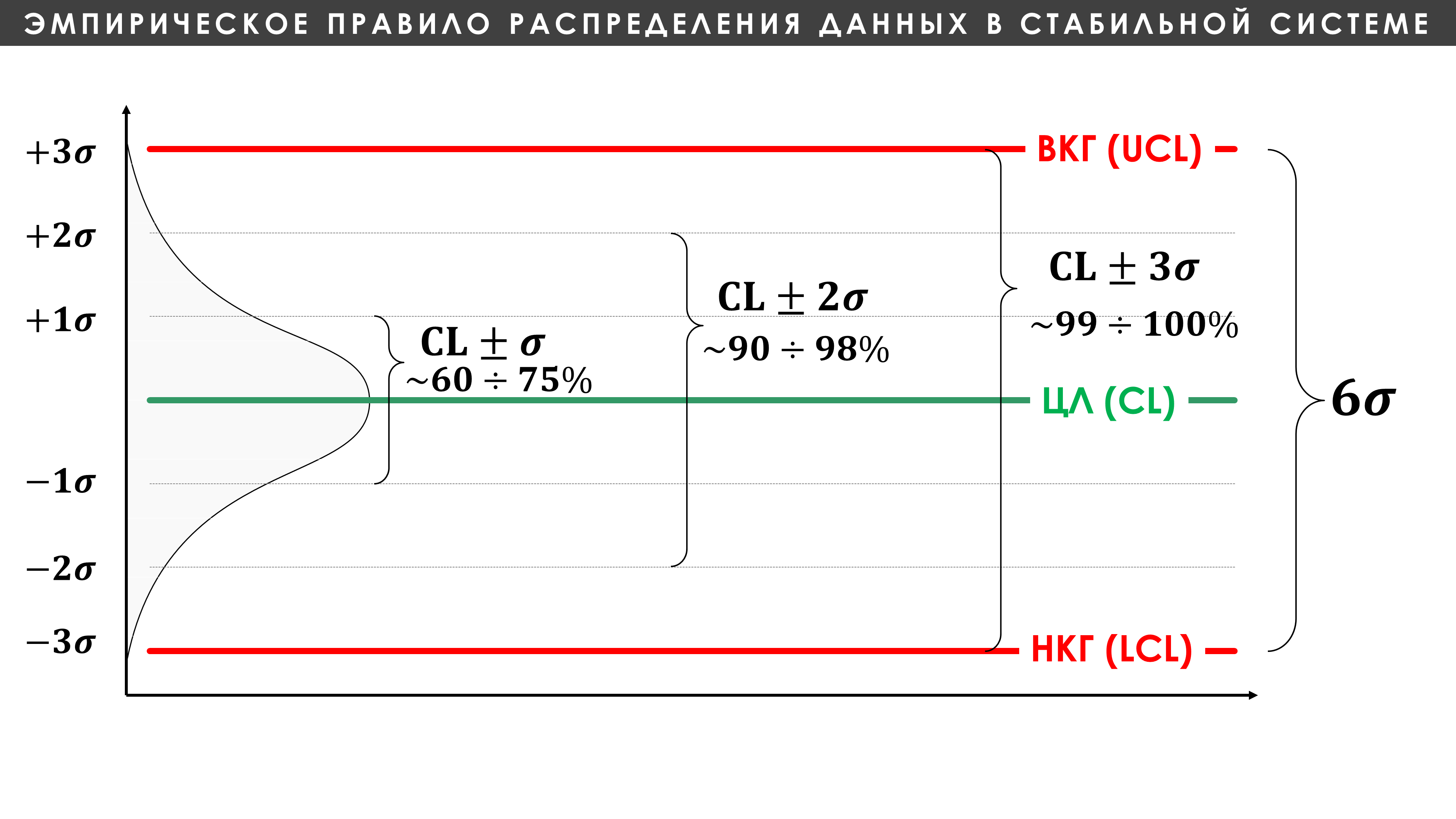
Figure 4. Rule of thumb for data distribution in a stable system. Shewhart control chart. The red lines, respectively, are the upper (Upper Control Limit, UCL, ВКГ) and lower (Lower Control Limit, LCL, НКГ) control limits. Green line - Central Line (CL, ЦЛ) - average value.
"The rule of thumb provides us with a useful way of describing data using a measure of position and a measure of dispersion. If given a homogeneous set of data, then:
1) approximately 60–75% of the data are within one sigma unit on either side of the mean;
2) approximately 90 to 98% of the data lie within two sigma units of the mean;
3) approximately 99–100% of the data are no more than three sigma units away from the average.
The sigma unit (σ) is a measure of the scale of the data. General scattering statistics can be converted to (σ)-units using published formulas*."
* Formulas for calculating σ-units, see [11.1] GOST R 50779.42-99 (ISO 8258-91) - Note Sergey P. Grigoryev
Video 3. Rule of thumb for the distribution of values in a stable system. Shewhart's control chart for the Galton board experiment. The red lines, respectively, are the upper (Upper Control Limit, UCL, ВКГ) and lower (Lower Control Limit, LCL, НКГ) control limits. Green line - Central Line (CL, ЦЛ) - average value.
Video 3 with the rule of thumb for the distribution of values in a stable system proves the lack of scientific and practical meaning in the statement that the [+/- 2σ] boundaries are warning boundaries. A small part of homogeneous values should be outside these boundaries of a stable process in any case. And the actual signals are the points on the Shewhart control chart determined in accordance with Western Electric zonal criteria .
Moreover, [4] Donald Wheeler, in Statistical Process Control: Business Optimization Using Shewhart control charts, demonstrates six theoretical data distributions, and for all distributions the [+/- 2σ] bounds are non-prejudicial. For a uniform distribution - these could be the action limits, and for those remaining outside the normal distribution, only the [- 2σ] limit could be the lower action limit (lower control limit, LCL), but in the real world we never know the true model ( shape) of the distribution of the analyzed parameter. See the picture below.

Figure 5. Six theoretical data distributions with arrows indicating boundaries [+/- 2σ].
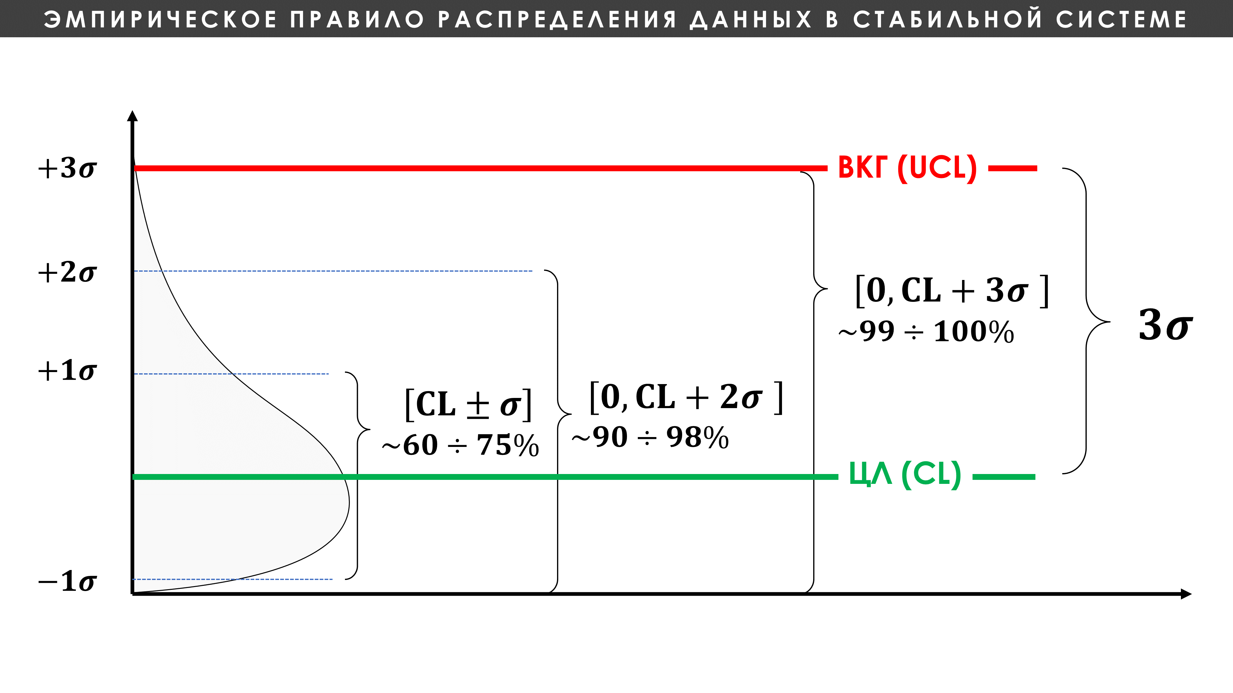
Figure 6. An example of a special case of applying an empirical rule for data distribution in a stable system for a process with one control limit. Shewhart control chart. The red line is the top (Upper Control Limit, UCL, ВКГ). Green line - Central Line (CL, ЦЛ) - average value.
“Kanban, or just-in-time, is a natural consequence of achieving a state of statistical control for product quality measures, which in turn leads to achieving statistical control for the speed of the production process.”
Process control limits “know nothing” about the tolerance limits (specification requirements) against which product defects are determined. Product defects are determined by artificially established tolerance limits or specifications. Push the specification boundaries beyond the control limits of a statistically controlled process and you have “zero defects” or “defect-free manufacturing.” There were “zero defects”, bring the specification boundaries closer by placing them inside the control limits of the Shewhart chart - here you have guaranteed “defects”, the probable number of which can be easily predicted by the empirical rule of data distribution in a stable system.
What actions should not be taken, and what actions should really be taken in relation to the process that produces defective products, is presented in the article: Correct and incorrect ways to use tolerance fields. Should products be sorted according to tolerance margins for defective and non-defective, or should we try to customize the process? .
“Meeting tolerances is not enough.
Moreover, there is no way to know whether tolerances will be maintained unless the process is in a state of statistical control. Until special causes are identified and ruled out (at least those that have appeared so far), no one can predict what the process will produce in the next hour.
Reliance on inspection (the only alternative) is dangerous and costly. Your process may work well in the morning and produce out-of-tolerance items in the afternoon.
Calculated tolerances are not boundaries that determine how to proceed. In fact, large losses occur when the process is constantly adjusted in one way or another to meet tolerances."
Statistically uncontrollable (unpredictable) process state

Figure 7. [4] Demonstration of data distribution and corresponding control XbarR-chart (XR map) of subgroup means and ranges for a time-varying process that is in a statistically uncontrollable state (unstable process). The red lines, respectively, are the upper (Upper Control Limit, UCL, ВКГ) and lower (Lower Control Limit, LCL, НКГ) control limits. Green line - Central Line (CL, ЦЛ) - average value.
The four points in the area of each histogram (bell-shaped curves) in Figure 5 are individual values and represent one subgroup of data of size n=4. The points in the mean Xbar control chart (top graph) represent the means of each subgroup of points from the corresponding histograms. The points on the subgroup range R chart (bottom graph) represent the subgroup range (the difference between the maximum and minimum value in each subgroup). All points on the graphs of the XbarR control chart are placed from left to right as values are formed over time.

Figure 8. Demonstration of data distribution for an unpredictable (statistically uncontrollable) process. As an example, the zones of the classic two-sided tolerance field are shown: the green zone is the tolerance field, the red zones are outside the tolerance field. The size of the tolerance field is chosen conditionally.
Video 4. Galton board experiment explaining the role of variability using the example of a statistically uncontrollable process that periodically changes its position relative to the tolerance zone. LSL (Lower Specification Limit) - lower limit of the tolerance field, USL (Upper Specification Limit) - upper limit of the tolerance field. The size of the tolerance field is chosen conditionally.
A statistically unstable (unpredictable, uncontrollable, unstable) process state can be identified using Shewhart control charts. This is the worst state for any process.
When control charts show signs of process instability, it is only then that immediate process intervention is required to identify and correct the specific causes of the instability.
"If a system is not in a state of statistical control, it is difficult to measure the effect of change. More precisely, if there is no control, only catastrophic results will be noticeable."
System changes made to an uncontrolled process are likely to be of little benefit to process improvement and will not be economically feasible. Moreover, if the process into which changes are planned to be made in order to improve it is in a statistically uncontrollable state, it will not be possible to reliably measure the effect of such changes.
First of all, it will be necessary to bring the process into a statistically stable state, which in itself always leads to a significant economic effect and does not require additional expenses.
Setting a specific numerical goal for an unpredictable process is more like profanity.

Figure 9. A numerical goal for an unpredictable process is like reading tea leaves. Shewhart's control chart for a statistically uncontrollable (unstable) process.
The red lines, respectively, are the upper (Upper Control Limit, UCL, ВКГ) and lower (Lower Control Limit, LCL, НКГ) control limits. Green line - Central Line (CL) - average value, 𝝈 - measure of data dispersion (calculated value inherent in a specific unique process).
Literature:
- [11] GOST R ISO 7870-1-2011 (ISO 7870-1:2007), GOST R ISO 7870-2-2015 (ISO 7870-2:2013) - Statistical methods. Shewhart control charts. Download (PDF) 7870-1 , 7870-2 .
- [11.1] GOST R 50779.42-99 (ISO 8258-91) Statistical methods. Shewhart control charts (version before the release of GOST 7870-1, 7870-2) - we at DEMING.PRO prefer this version. Download (PDF) 50779.42-99 .
- [12] GOST 51814.3-2001 – Quality systems in the automotive industry. Methods of statistical process control. Download (PDF) 51814.3 .
Article: Rules for determining lack of controllability using control charts .
The short video below provides a roadmap for a cost-effective method of improving a process to the point where the process operates so tightly within specified tolerances that it produces no defective products at all. This process goal easily neutralizes the uncertainty of the measured values due to the error of the measurement system, which in turn must be in a stable state, since there will be no boundary values placed at the tolerance boundaries.
Material on boundary values is presented in the article: Is the product meeting the specification (approval) actually meeting the specification? Are defective products really defective? .
Video 5. What needs to be done to improve processes?
Symbols of elements in the video: НГД and ВГД - lower and upper tolerance limits, respectively (Eng, LSL and USL); m0 - nominal tolerance field; НГП and ВГП - lower and upper natural boundaries of the process (English LNPL and UNPL); CL - central line of the process (average of the process).
See description Taguchi quality loss functions , giving operational definition world class quality.
"The concept of 'fine-tuning on target with minimal variance' has defined world-class quality for the last thirty years! And the sooner you make this principle the rule of your life, the faster you will become competitive!"
Many companies have understood and adopted the concept of world class quality as succinctly formalized by Donald Wheeler, here are some examples:

Figure 10. Renault F-1 racing car.
“We ended up working with ultra-low viscosity fluids, much lower than any other product the Renault F1 team had used before, combined with smart technology in the additive systems. By upgrading their bearing system to tighter tolerances, they were able to reduce friction to a level where the engine could go a little further, run a little more."
Note!
In order for Castrol to be able to use ultra-low viscosity grease, the bearing manufacturer had to achieve lower tolerance production of bearings (due to the retention of ultra-low viscosity grease in the bearing). This once again confirms that significant innovation can only be achieved through the cooperation of all parties involved, as Edwards Deming constantly reminded, speaking about the need to expand the boundaries of the system for its better optimization.
Diagnosing actual changes in the process
Below is a film about a method for quickly diagnosing changes in a process (system), both positive and negative, using the Shewhart control chart.
Video 6. A method for quickly diagnosing changes in a process using Shewhart control charts. The red lines, respectively, are the upper (Upper Control Limit, UCL, ВКГ) and lower (Lower Control Limit, LCL, НКГ) control limits. Green line - Central Line (CL, ЦЛ) - average value.
See description of experiments "funnel and target" And "red beads" - Excellent demonstrations of the nature of variation and common management practices.