Correct and incorrect ways to use tolerance fields. Should products be sorted according to tolerance margins for defective and non-defective, or should we try to customize the process?
Article: [26] DONALD J. WHEELER: "Right and Wrong Ways to Use Specifications. Sorting or Adjusting?"
Translation, notes and additional graphic materials with explanations: Scientific Director of the AQT Center
Sergey P. Grigoryev
, using materials kindly provided to him by Donald Wheeler.
Free access to articles does not in any way diminish the value of the materials contained in them.
In this article, we'll look at the history and purpose of tolerance fields, and look at two common ways to use them in practice. Using simple examples, I will illustrate the correct and incorrect ways to use tolerance fields (specifications).
Note Sergey P. Grigoryev: The article demonstrably demonstrates that the operational adjustment of the process by the machine operator relative to the tolerance fields makes sense only for processes that are unstable and/or not centered in the tolerance field, while the correction of stable and well-centered processes in the tolerance field leads to even greater variability (a greater spread of data around the mean), which deprives workers of understanding “what is happening?” when trying to improve the quality of the parts he produces.
Voice of the customer
About 220 years ago, Eli Whitney created a cotton gin with replaceable parts. The use of interchangeable parts was a technological breakthrough of the time. Shortly after his success with the cotton gin, Whitney received a contract to supply the U.S. Army with muskets that had interchangeable parts. In an attempt to produce a large number of parts so that they could be used interchangeably, he immediately discovered a fact that has haunted every production since: no two things are alike.
So instead of making things the same, they had to be content with making them similar. Once they accepted this, the question immediately arose: “how similar are similar enough parts?” In an attempt to answer this question, technical conditions (tolerance fields, specifications) were created. It was obvious that minor deviations could be tolerated as the parts would still function. However, as variations increase, there will come a point when it will be cheaper to discard the part than to try to use it. And the tolerance fields (specifications) were intended to determine this loss cut-off point.
Two hundred years ago, the economy of mass production was so great that large amounts of waste could be tolerated. By the 1840s, the gauge (pass-fail) tool was invented. By the 1860s, this had evolved into the "go-no-go gauge" which allowed large quantities of parts to be sorted economically into good and bad parts. This 1860s technology is still in use today. Tolerance fields were created to separate acceptable product from unacceptable product. Whenever a product stream contains nonconforming elements that can be identified by nondestructive testing, the use of 100 percent testing remains a reasonable strategy when it can be done in an economically feasible manner. Once you've burned your toast, what can you do besides clean up the burnt bits?
Example
Figures 1 and 2 show the 100 final test values along with their histogram and the Shewhart X-map for the individual values. These values are derived from a manufacturing operation at one of my client's plants. The tolerance bands for these values range from 67 to 71. The histogram shows that this process has only 34 percent yield, while the X-map shows that this process operates unpredictably. The tolerance margin allows us to differentiate between conforming and non-conforming items, but a yield of 34 percent is unacceptable.
Do you need to do something?
One popular course of action is to try to improve the output by making appropriate process adjustments. Let's assume that we can adjust the process after each measurement result of a part selected for inspection (test) and that each adjustment will affect subsequent products produced. We will use the tolerance limits of 67 and 71 to determine the dead zone for our adjustments. That is, we will adjust the process only when we receive an inappropriate test result. If, say, we have a test result of 65, then we will adjust the process up by 4 to target the process to an average tolerance value of 69, and if we have a result of 75, then we will adjust the process down by 6. However, if we have test result is 67, 68, 69, 70 or 71, we will not make any changes to this process. We will further call this type of adjustment “P-controller”.
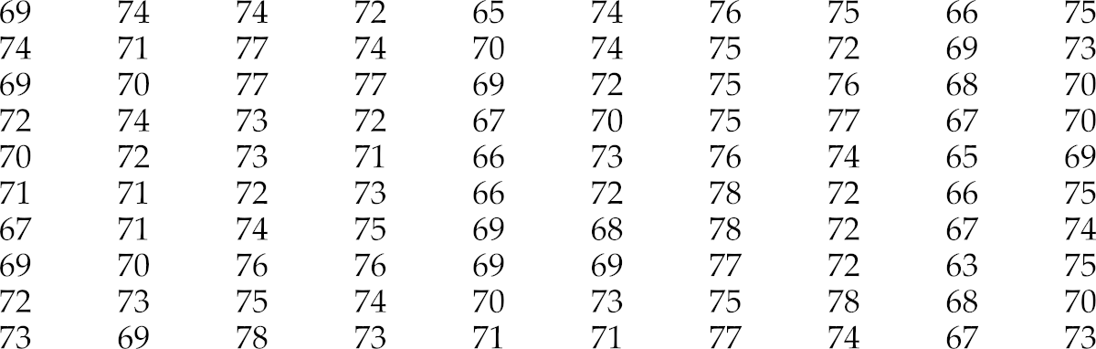
You can download the data in the sorted list in CSV format to build your own XmR control chart: download .
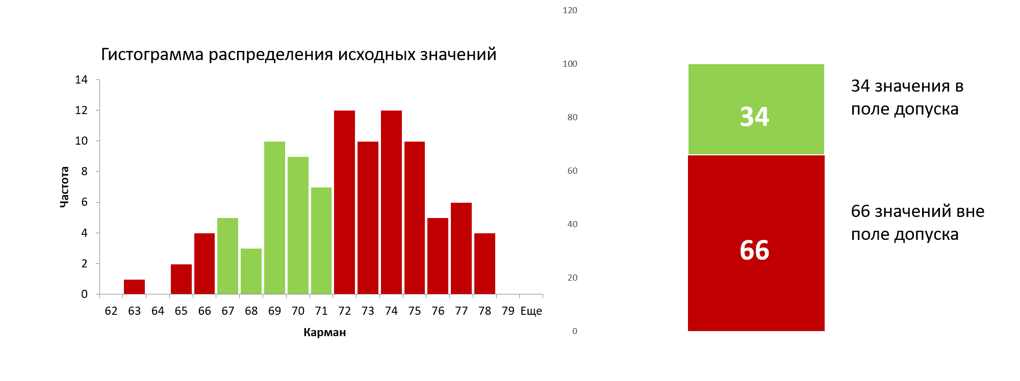
Figure 1: Histogram of the distribution of 100 initial values of an unstable and poorly centered process before adjustment.
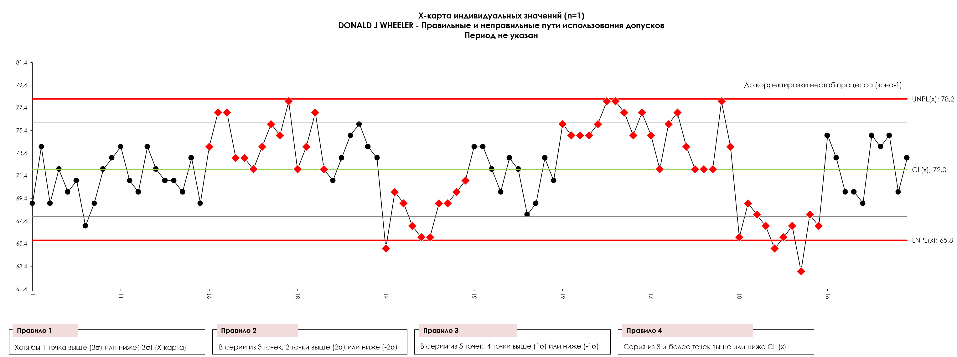
Figure 2: X-map of individual values (process voice) 100 initial values of an unstable and poorly centered process before operator correction. The red lines, respectively, are the upper and lower natural boundaries of the process, the green line is the central line (average) of the process. Red dots (series of dots) are signals of the presence of special causes, indicating a statistically uncontrollable state of the process. The drawing was prepared using our developed “Shewhart control charts PRO-Analyst +AI (for Windows, Mac, Linux)” .
The animated Figure 2 below shows how the adjustment procedure will work with the original data in Figure 1. For example, an initial value of 69 will not cause subsequent values to be adjusted. A second value of 74, plus a zero adjustment to the previous measurement, results in an adjusted value of 74. This results in an adjustment of -5 to a process target of 69. A third value of 69 plus a previous measurement adjustment of -5 gives an adjusted third value of 64. This results in an adjustment of +5 next process values, etc.
Figure 3: Animation of the changing 100 initial values as an unstable and poorly centered process is corrected. USL is the upper limit of the tolerance, Target is the nominal value of the tolerance field, LSL is the lower limit of the tolerance field.
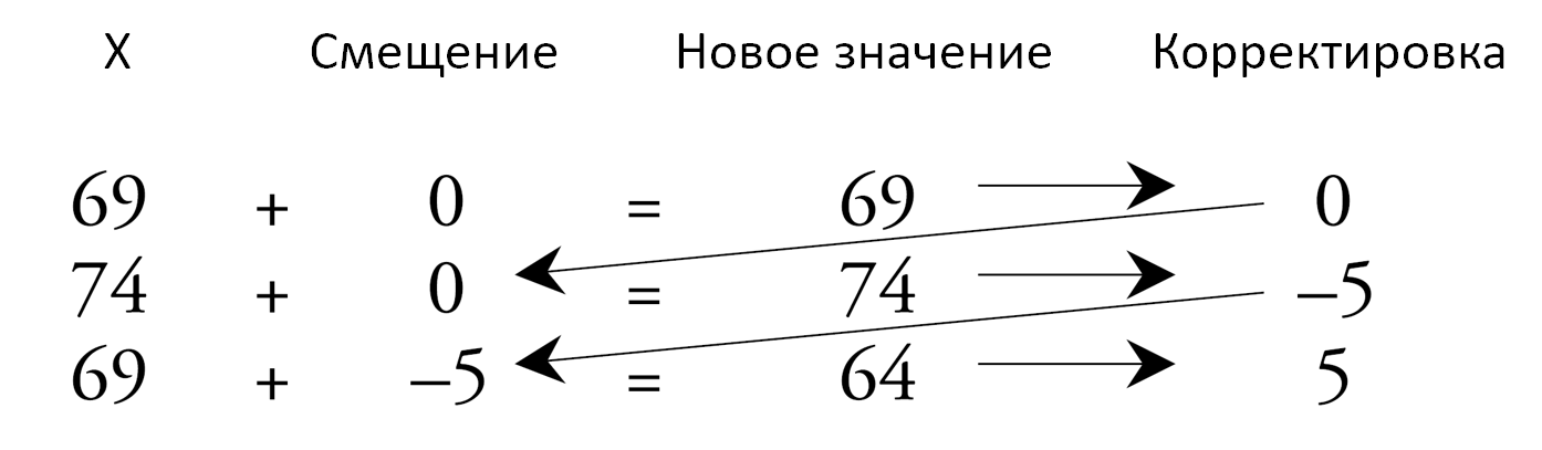
Figure 4: Rule for adjusting the process by measuring a “defective” part.
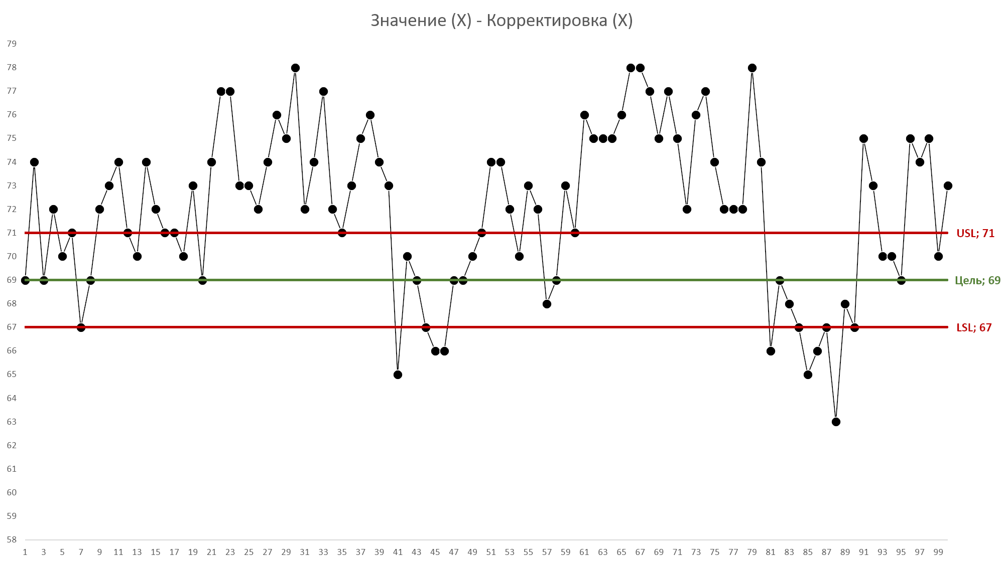
Figure 5: Graph of 100 (one hundred) initial values before adjusting an unstable and poorly centered process against tolerance fields (voice of the client). USL is the upper limit of the tolerance, Target is the nominal value of the tolerance field, LSL is the lower limit of the tolerance field.
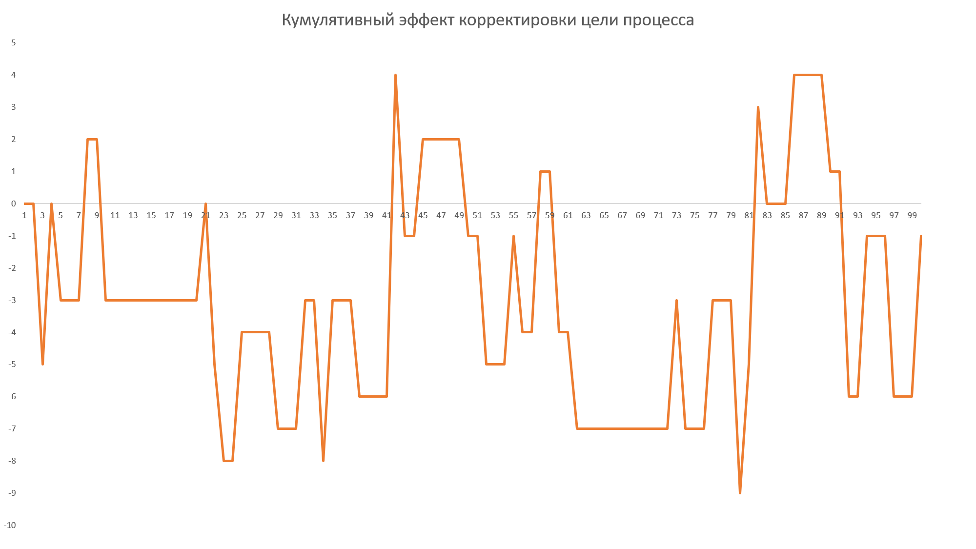
Figure 6: Cumulative effect of adjusting an uncontrolled and poorly centered process.
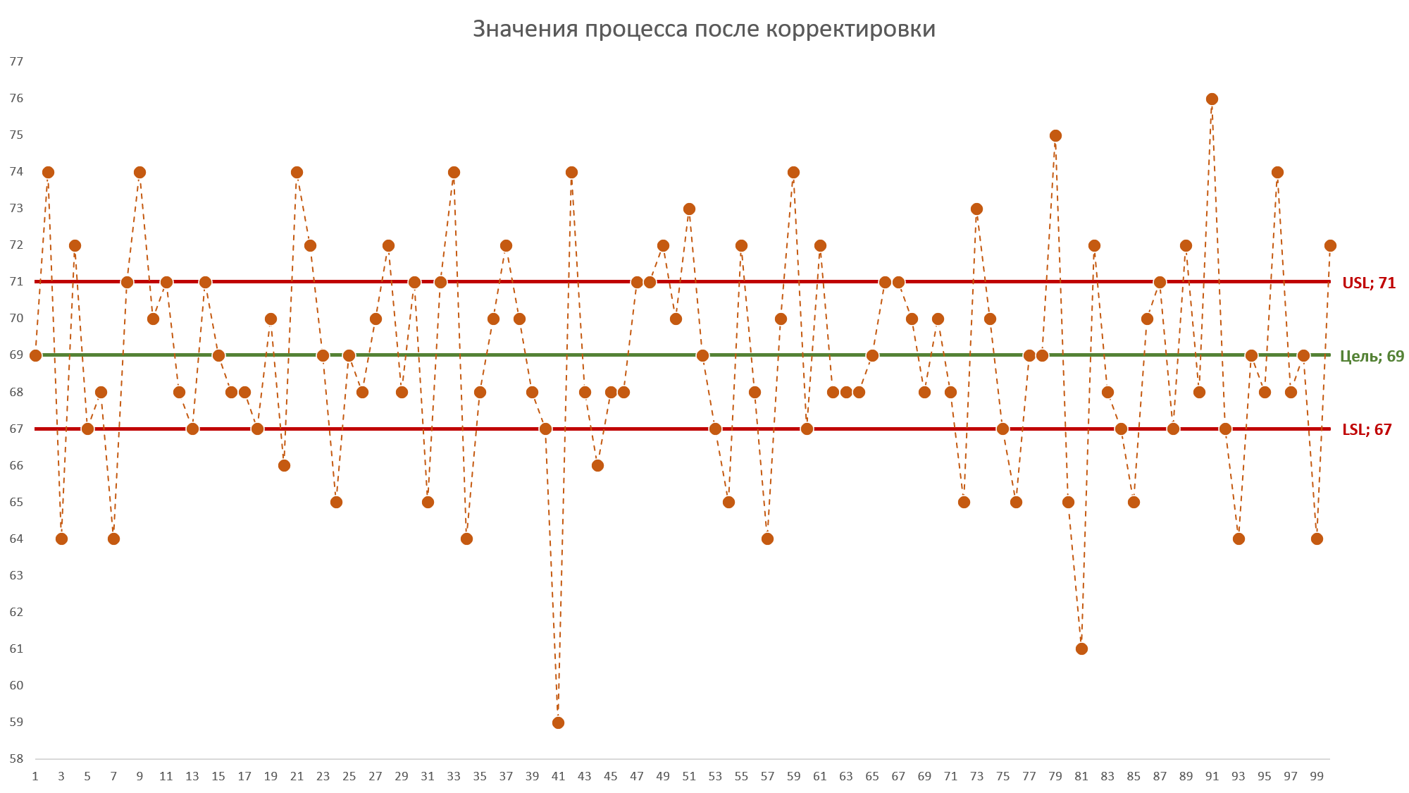
Figure 7: Resulting data from an uncontrolled and poorly centered process after conversion by a P-controller using tolerance bands as a deadband. USL is the upper limit of the tolerance, Target is the nominal value of the tolerance field, LSL is the lower limit of the tolerance field.
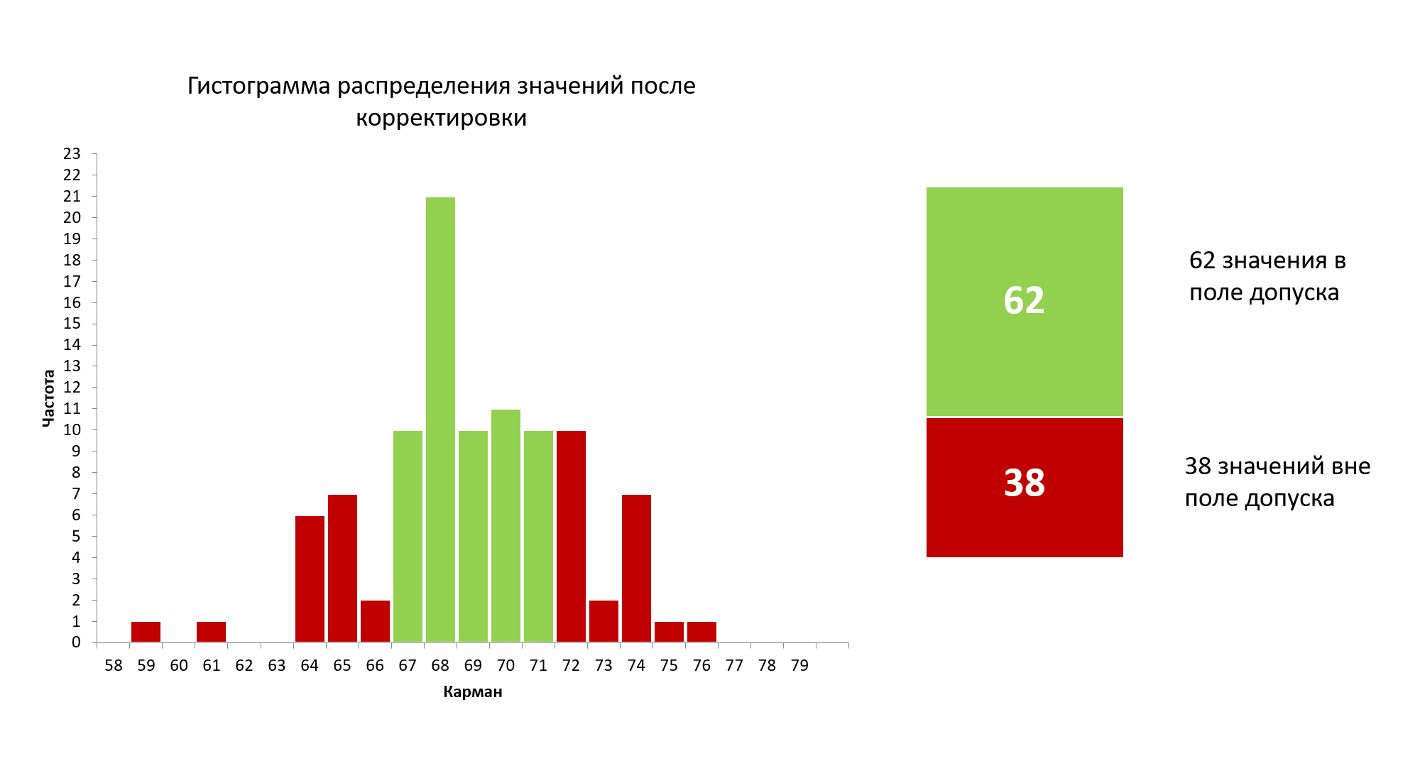
Figure 8: Histogram of the distribution of 100 new values after correcting for an unstable and poorly centered process.
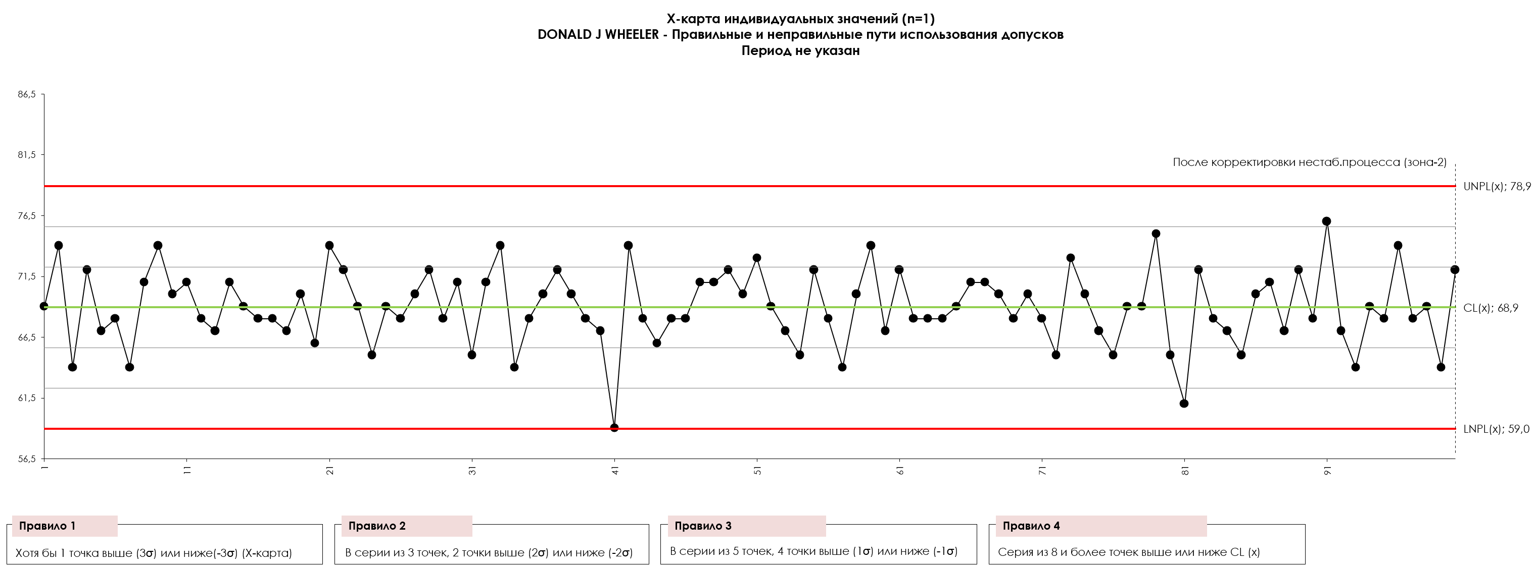
Figure 8.1.: X-map of individual values (process voice) 100 values after operator correction of the unstable and biased (non-centered) process shown in Figure 2. demonstrates a statistically stable state. The drawing was prepared using our developed “Shewhart control charts PRO-Analyst +AI (for Windows, Mac, Linux)” .
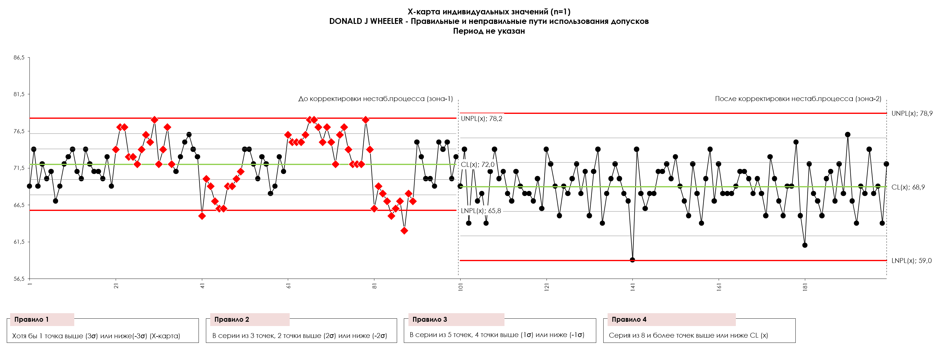
Figure 8.2.: X-map of individual values (process voice) of 100 values before (zone-1) and after (zone-2) correction of an unstable and biased (non-centered) process demonstrates a statistically stable state. The drawing was prepared using our developed “Shewhart control charts PRO-Analyst +AI (for Windows, Mac, Linux)” .
So how did we cope? The P-controller using tolerance limits to determine the dead zone boosted yield from 34 percent to 62 percent. A very impressive improvement. This happened because this process was not concentrated in the tolerance zone and was controlled unpredictably. As a result of these two aspects of the data shown in Figure 2, many of the thirty-two (32) adjustments were actually needed for improvement, and therefore the P-controller improved performance.
However, a yield of 62 percent was not all that the process was capable of. It could have been better. Once we identified the special causes of the exceptional variation shown in Figure 2 and took steps to control those special causes in production, we ended up with the process shown in Figure 9 (below).
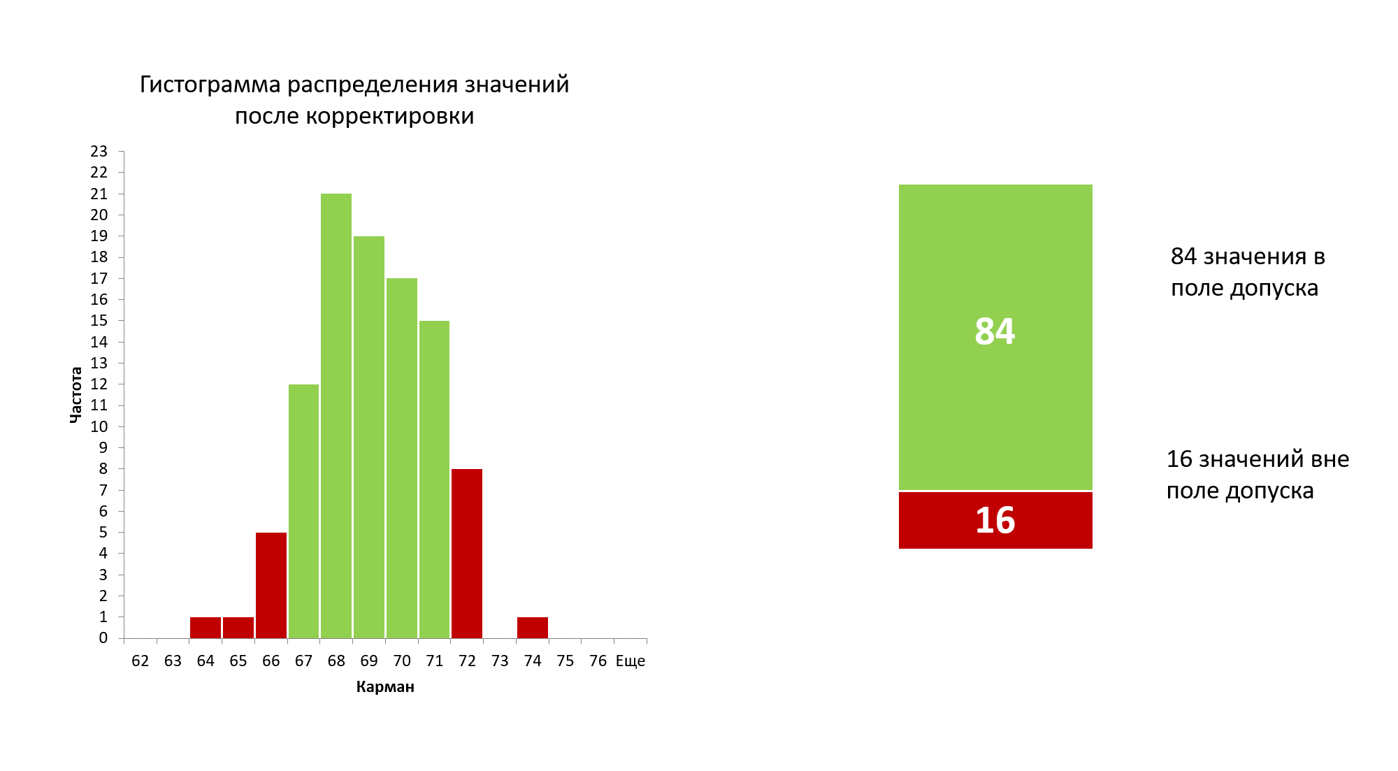
Figure 9: Histogram of the distribution of 100 new values after removing previously identified special causes of variability.
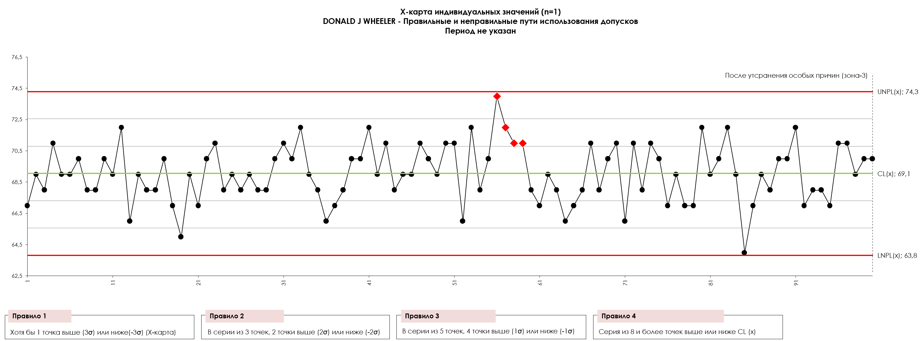
Figure 10: X-map of individual values (process voice) 100 values. The process in the figure works quite predictably. Previously manifested special causes of variation have been eliminated, with the exception of a series of points 55, 56, 57, 58, 59, 60 in which possibly new special causes of variability have appeared. UNPL is the upper natural control limit of the process, LNPL is the lower natural control limit of the process, CL is the center line (average). The drawing was prepared using our developed
“Shewhart control charts PRO-Analyst +AI (for Windows, Mac, Linux)”
.
Note Sergey P. Grigoryev: You can download the stabilized process data in a sorted list in CSV format to independently build a control XmR-chart:
download
.
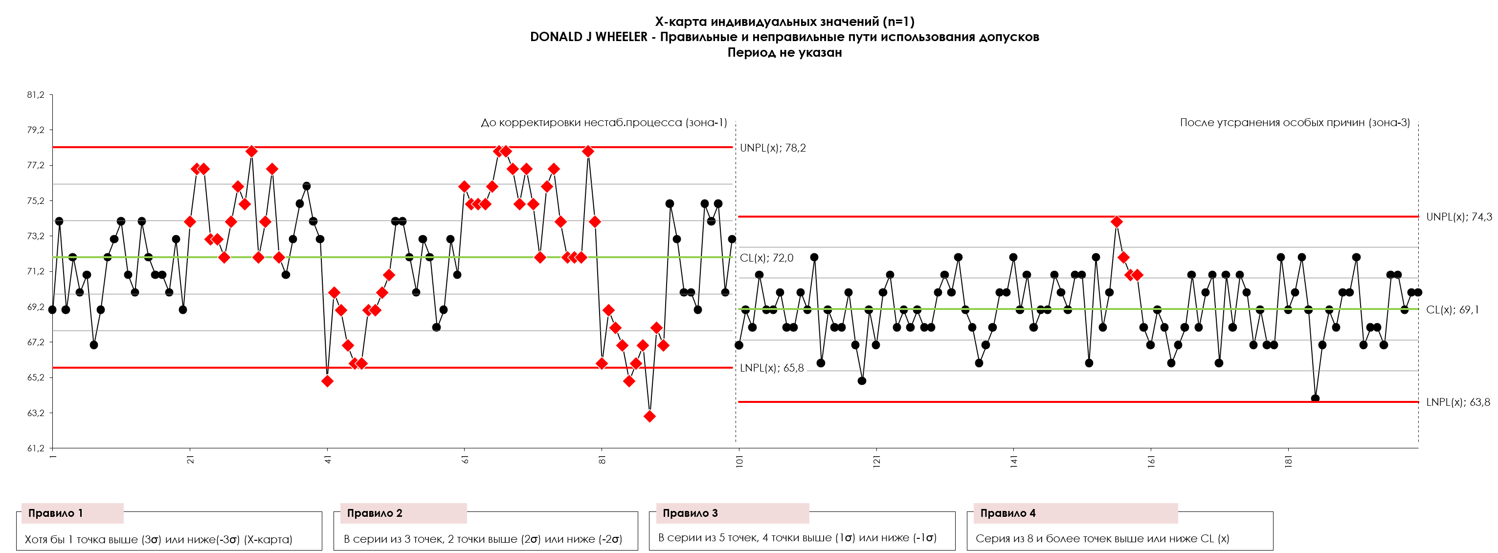
Figure 10.1: X-map of individual values (process voice) of 100 values before eliminating the special causes of variability in an unstable process (Zone-1) and after (Zone-3). UNPL is the upper natural control limit of the process, LNPL is the lower natural control limit of the process, CL is the center line (average). The drawing was prepared using our developed “Shewhart control charts PRO-Analyst +AI (for Windows, Mac, Linux)” .
When they began to manage this process predictably and to its target (tolerance value), their yield rose to 84 percent. This is the full potential for this process in its current state. An 84 percent yield is not some impossible goal, but simply what the process is capable of producing when operating at its full potential. Predictive work will minimize variation in process outputs, while work to process objectives will maximize the conformity of the manufactured product.
Let's try to improve a stable process using the same method
But the process still does not produce 100 percent compliant products. Can't we do something about the 16 percent non-conforming product? Well, what if we apply a P-controller with a dead zone in the data tolerance field in Figure 10? When we do this, we end up with the data in Figure 11.
Figure 11: Animation of the changing 100 initial values as a stable and well-centered process is adjusted. USL is the upper limit of the tolerance, Target is the nominal value of the tolerance field, LSL is the lower limit of the tolerance field.
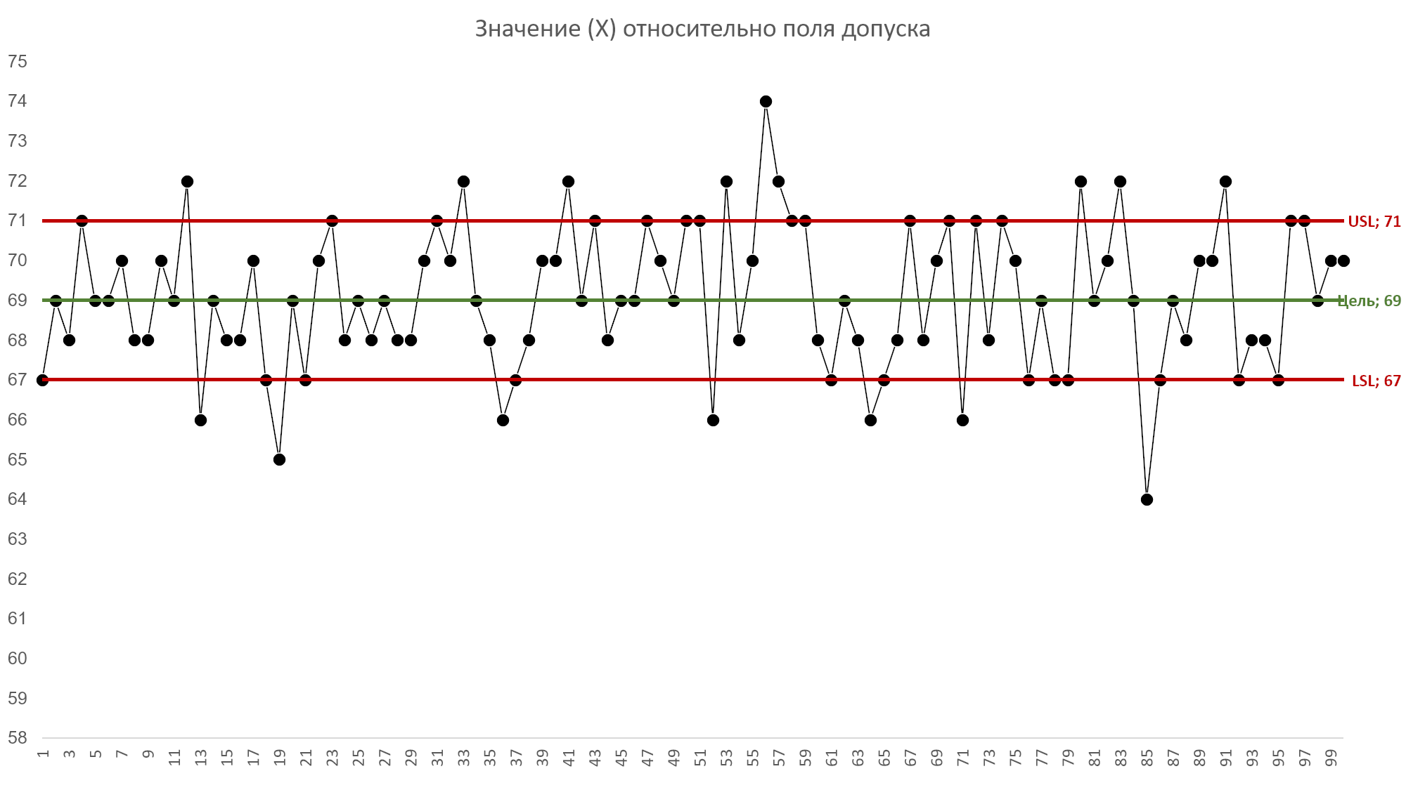
Figure 12: Plot of one hundred initial values before adjusting a stable and well-centered process against tolerance margins (voice of the customer). USL is the upper limit of the tolerance, Target is the nominal value of the tolerance field, LSL is the lower limit of the tolerance field.
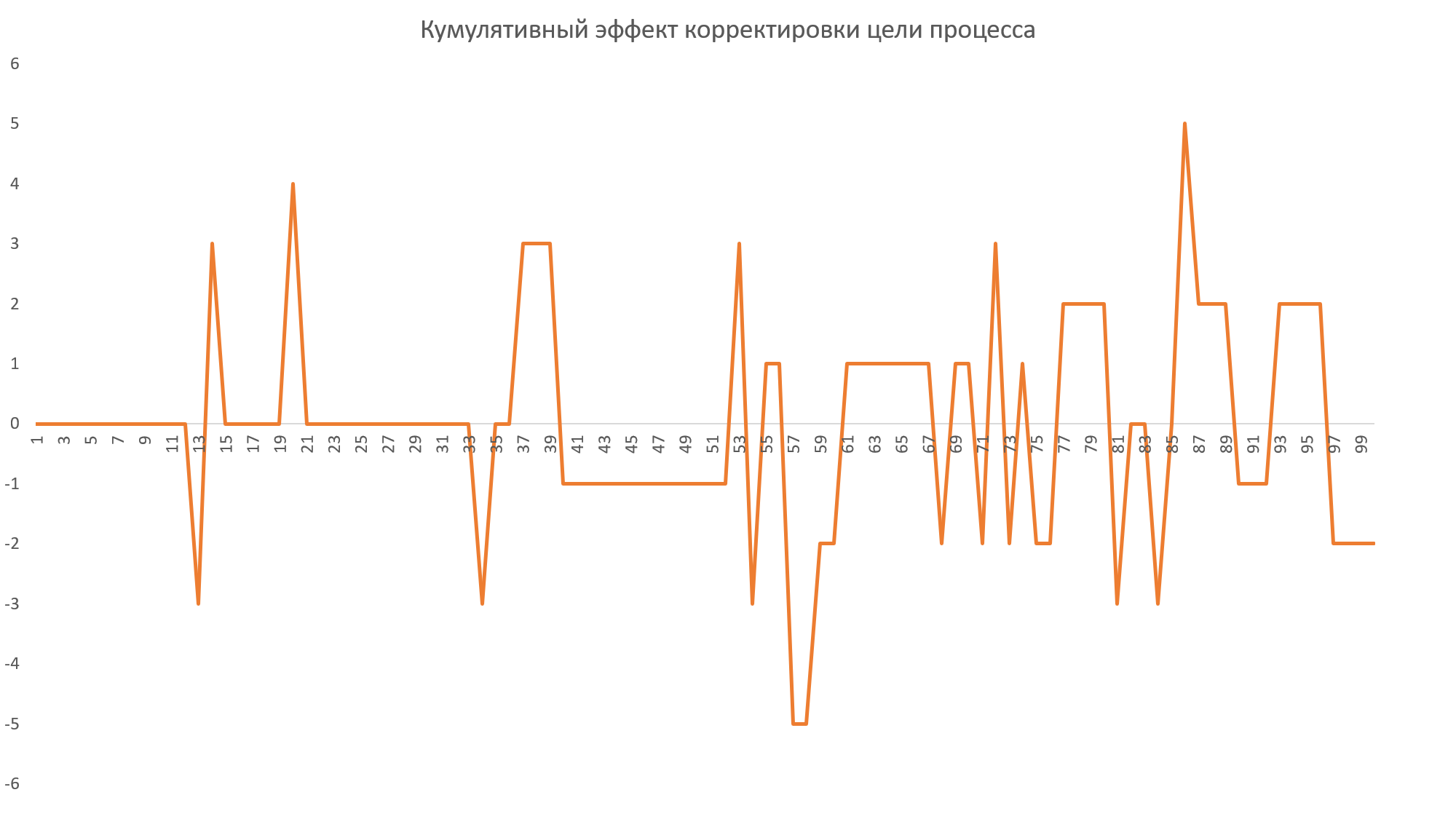
Figure 13: Cumulative effect of adjusting a stable and well-centered process.
Note by Sergey P. Grigoryev: Please note that the graph of the Cumulative Effect of Adjustments for a stable and well-centered process presented in Figure 13 differs in its symmetry about the (X) axis from the same graph for an unstable and uncentered process (Figure 6). Which in the case of Figure 13 suggests that in trying to adjust a stable and well-centered process, we were simply messing around with moving some values down and others up, only making things worse. “We wanted the best, but it turned out as always.” - V.S. Chernomyrdin.
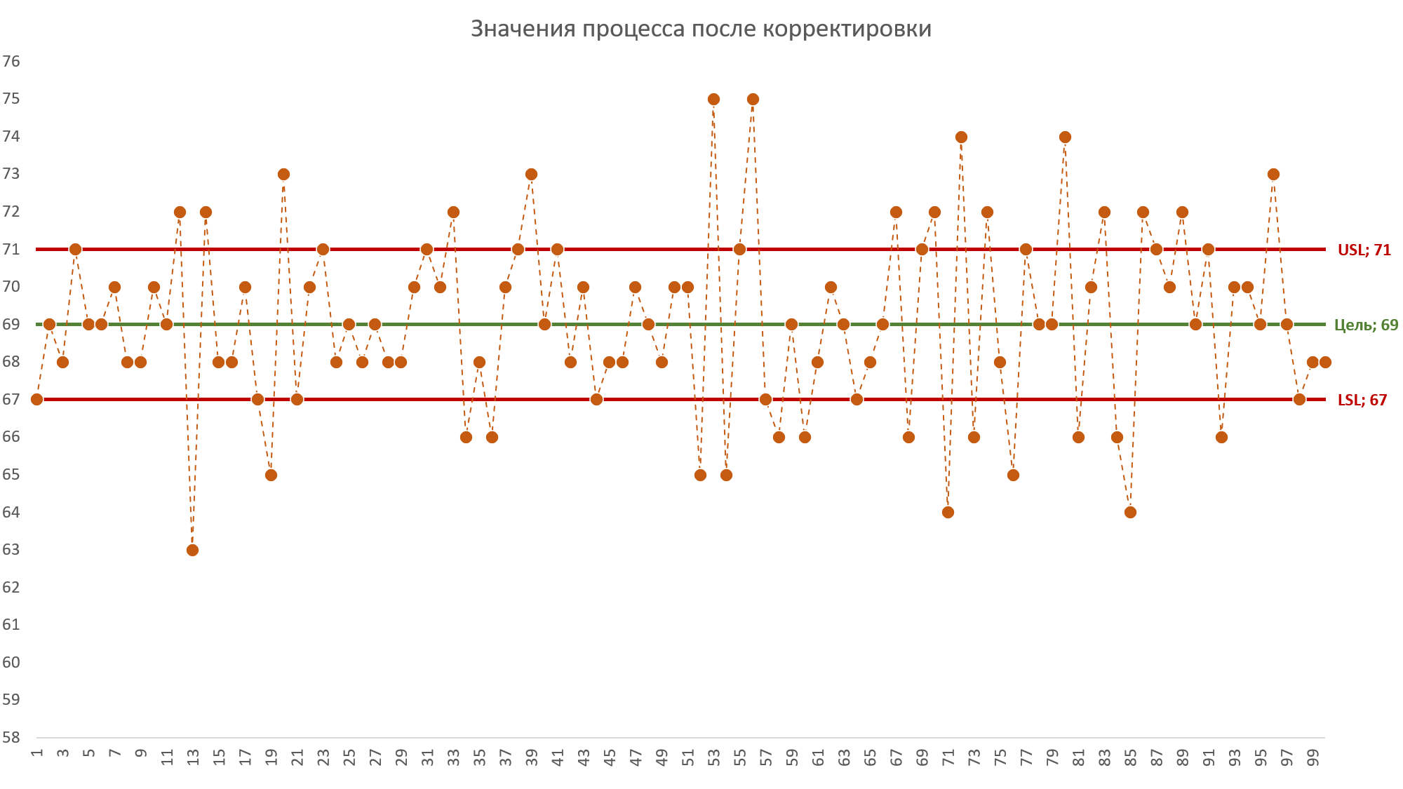
Figure 14: Resulting data from a stable and well-centered process after conversion by a P-controller using tolerance bands as a deadband. USL is the upper limit of the tolerance, Target is the nominal value of the tolerance field, LSL is the lower limit of the tolerance field.
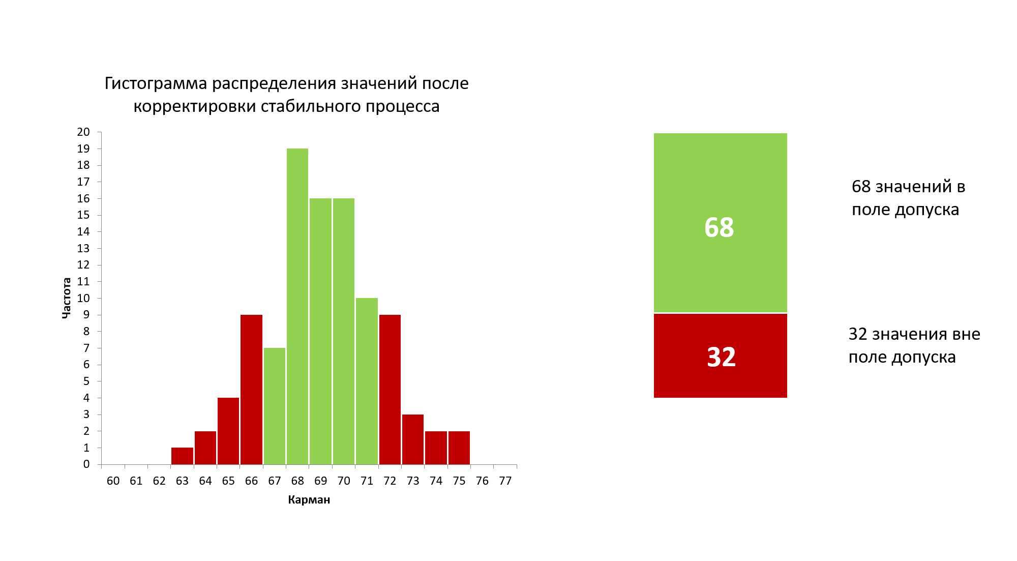
Figure 15: Histogram of the distribution of 100 new values after attempts to adjust a stable and well-centered process.
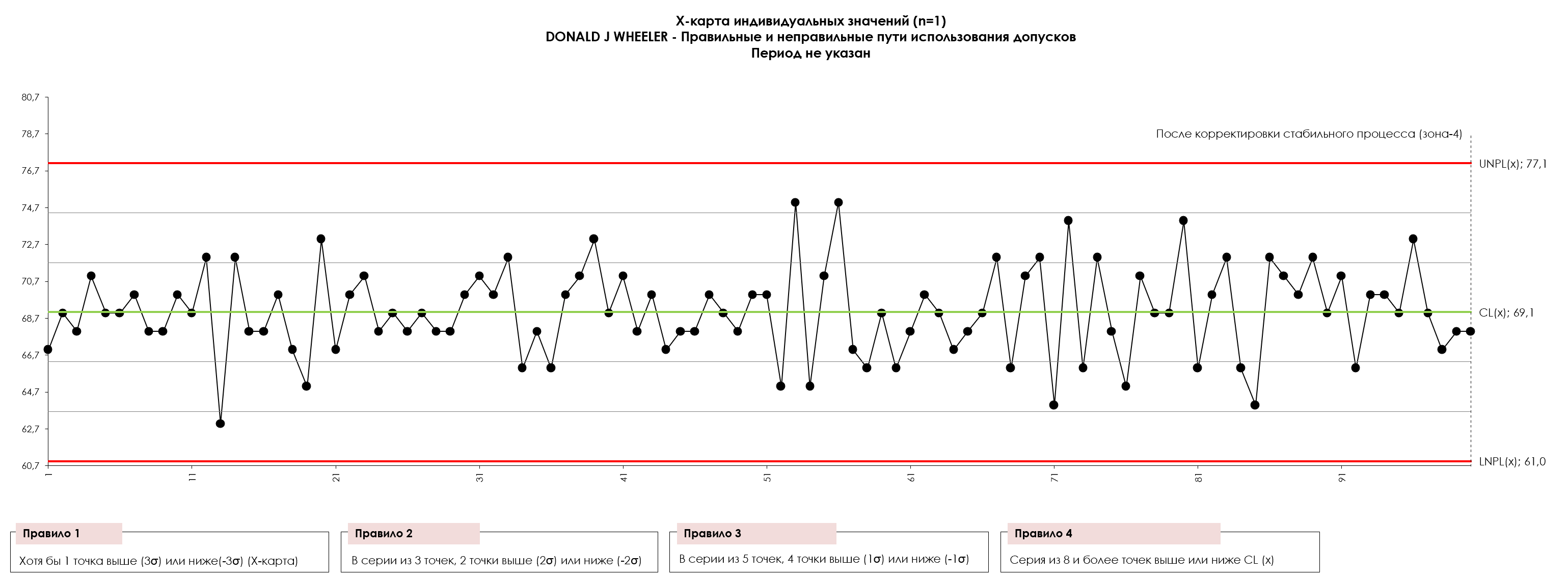
Figure 16. X-map of individual values (process voice) of 100 values after attempting to adjust a stable and well-centered process. UNPL is the upper natural control limit of the process, LNPL is the lower natural control limit of the process, CL is the center line (average). The drawing was prepared using our developed “Shewhart control charts PRO-Analyst +AI (for Windows, Mac, Linux)” .
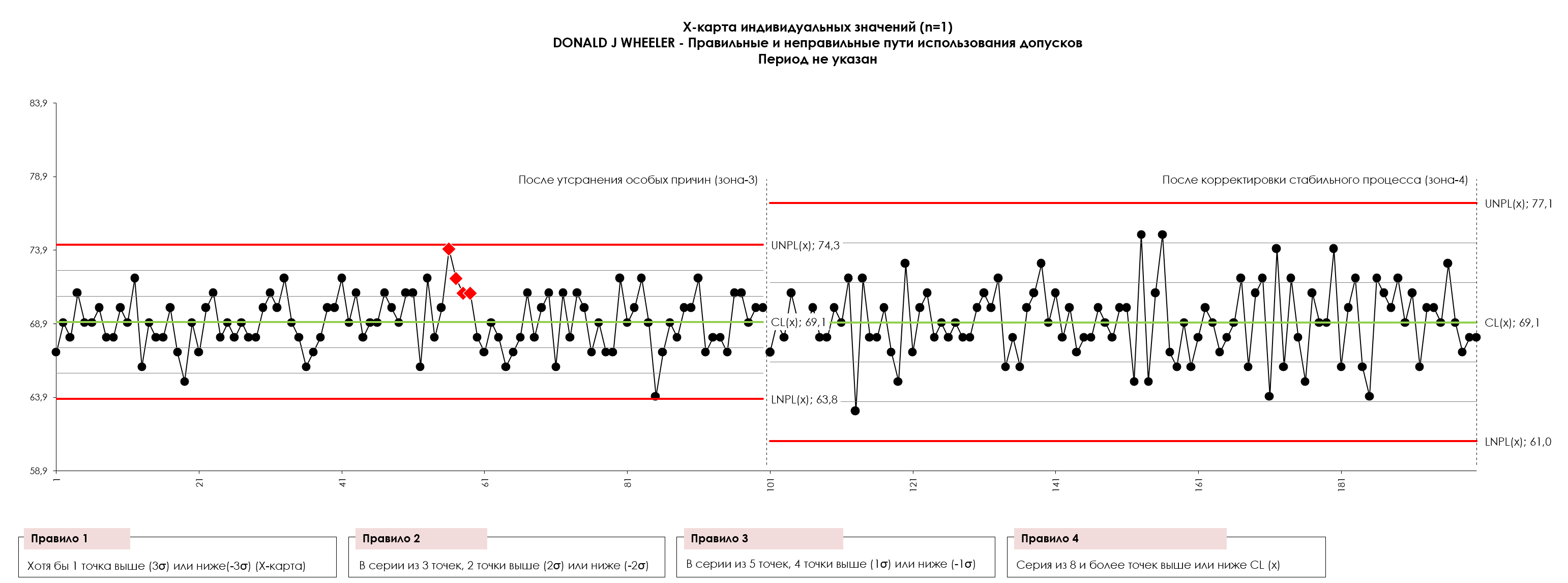
Figure 16.1. X-map of individual values (process voice) 100 values before (Zone-3) after (Zone-4) the operator's attempt to correct a stable and well-centered process. UNPL is the upper natural control limit of the process, LNPL is the lower natural control limit of the process, CL is the center line (average). The drawing was prepared using our developed “Shewhart control charts PRO-Analyst +AI (for Windows, Mac, Linux)” .
Here the P controller, using the tolerance band as a deadband, converted a process that had 84% compliance to another process with 68% compliance! The share of non-conforming products doubled from 16 to 32 percent.
Why did this happen? This was due to the P controller reacting to noise and making inappropriate adjustments. With just a few adjustments in the first case (Figure 2), the P-controller began to produce positive results, but ultimately the unnecessary adjustments took the process further away from the goal and made the situation worse.
Note by Sergey P. Grigoryev: In an attempt to improve a stable process, it was necessary to make 32 adjustments. The lost time for adjustments only worsened the situation with the same actions as in the first case (Figure 2). This can throw any highly skilled operator into a complete stupor. What do you think the operator will do in this case? Will management help him solve this problem? Oh, if only management could know this! The result of any attempts to correct a well-centered and stable process is explained in simple language in the experiment with funnel and target Edward Deming.
“We ourselves will destroy everything with our own persistent efforts.”
In Figure 2, the process was not centered in the tolerance field and behaved unpredictably. There, the P-controller, using the tolerance band as a dead band, really improved things. In Figure 14, this process was centered and predictable. There the P-controller simply added noise to the process which increased the variation in product flow and made things worse.
So, what conclusion have we come to? Can we use tolerance to regulate a process that is in a statistically uncontrollable state? While using a P controller using the tolerance band as a deadband may be better than doing nothing, it doesn't allow you to get the most out of your process.
Why is the P-controller ineffective when the process operates predictably and is centered within the tolerance range? Any manual and automated process control mechanisms are inherently reactive. Whether it is a simple P controller or a more complex PID controller, they cannot act until they receive a sensed signal. Because the original process was unpredictable and not centered within the tolerance, there were many real signals that the P controller caught. However, there were also some weak signals (noise) that the P controller responded to, resulting in unnecessary adjustments. If the dead zone is completely out of tune with the process voice, your process adjustment mechanism will result in too many adjustments. In either case, the result will be increased variability in the product flow. Using an automatic controller for a stable process usually results in greater variability than what the process is capable of when it is operating at its full potential.
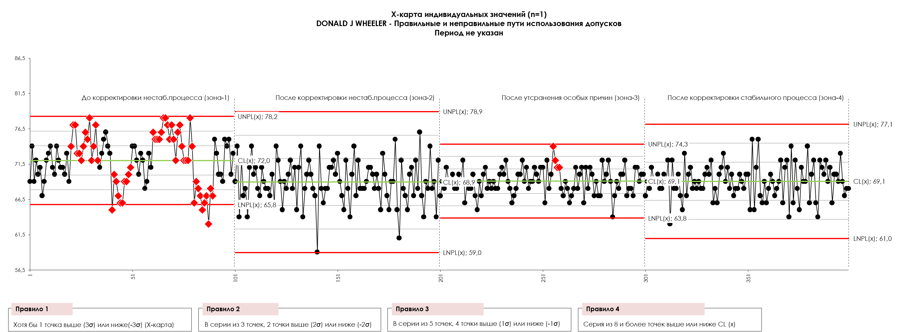
Figures 2; 8.1; 10; 16. X-map of individual values (process voice) 100 values for all cases discussed in the article above. UNPL is the upper natural control limit of the process, LNPL is the lower natural control limit of the process, CL is the center line (average). The drawing was prepared using our developed “Shewhart control charts PRO-Analyst +AI (for Windows, Mac, Linux)” .
See an example of operator intervention in the gas flow control process at an enterprise producing biogenic methane in the article: The concept of variability in process control .
Error of the first kind
- "But that means you won't react to values that are out of specification!"
Yes, the non-conforming values of 64, 65, 66 and 72, 73, 74 are part of what this process produces when it is running predictably and well centered within the tolerance. Let me repeat. As you can see from Figures 9 and 10, when this process is operating at its full potential, it will produce a product in the range of 64 to 74 (Y-axis). Taken one at a time, these values are not a signal that anything is wrong with the process, even though they may be out of specification. Tolerance fields are designed to sort suitable products from unsuitable ones. They are the voice of the customer, not the process. Clearance fields should never be confused with the voice of the process itself.
- “Are you saying that I should ignore non-conforming products?”
Non-conforming product must be rejected. But if your process is controlled predictably and tuned to target, the fact that an item is out of compliance does not tell you that a process adjustment is required.
Note by Sergey P. Grigoryev: In this case, further improvements will require systemic changes (change of raw materials, technology, equipment, tools, operator training, etc.).
Of course, process control cannot be controlled in a predictable and centralized manner without plotting a process behavior diagram (Shewhart XmR-chart of individual values), so there should be no guesswork involved. If you don't have a process behavior diagram, chances are at least 10 to 1 that you're running your process unpredictably. If this is the case, then an automatic process controller will only allow you to achieve a fraction of what your process is capable of.
Brief information
The modern quality movement is about learning how to stop burning toast. This doesn't mean we won't have to peel the toast from time to time; this means we move upstream to work on the process rather than sorting good material from bad at the end of the production line. Tolerance fields are still relevant, they still define the voice of the customer, but it is important to distinguish them from the voice of the process. While we do want the voice of the process to be aligned with the tolerance fields (voice of the customer), the tolerance fields do not provide the correct information about what needs to be done to get the full potential of your process.
Another simple case (Sergey P. Grigoryev)
I am sure that it is necessary to consider one more situation when the process is in a statistically stable (controlled) state, but is not centered in the tolerance field. In an example of such a process, 77 values are outside the tolerance range.
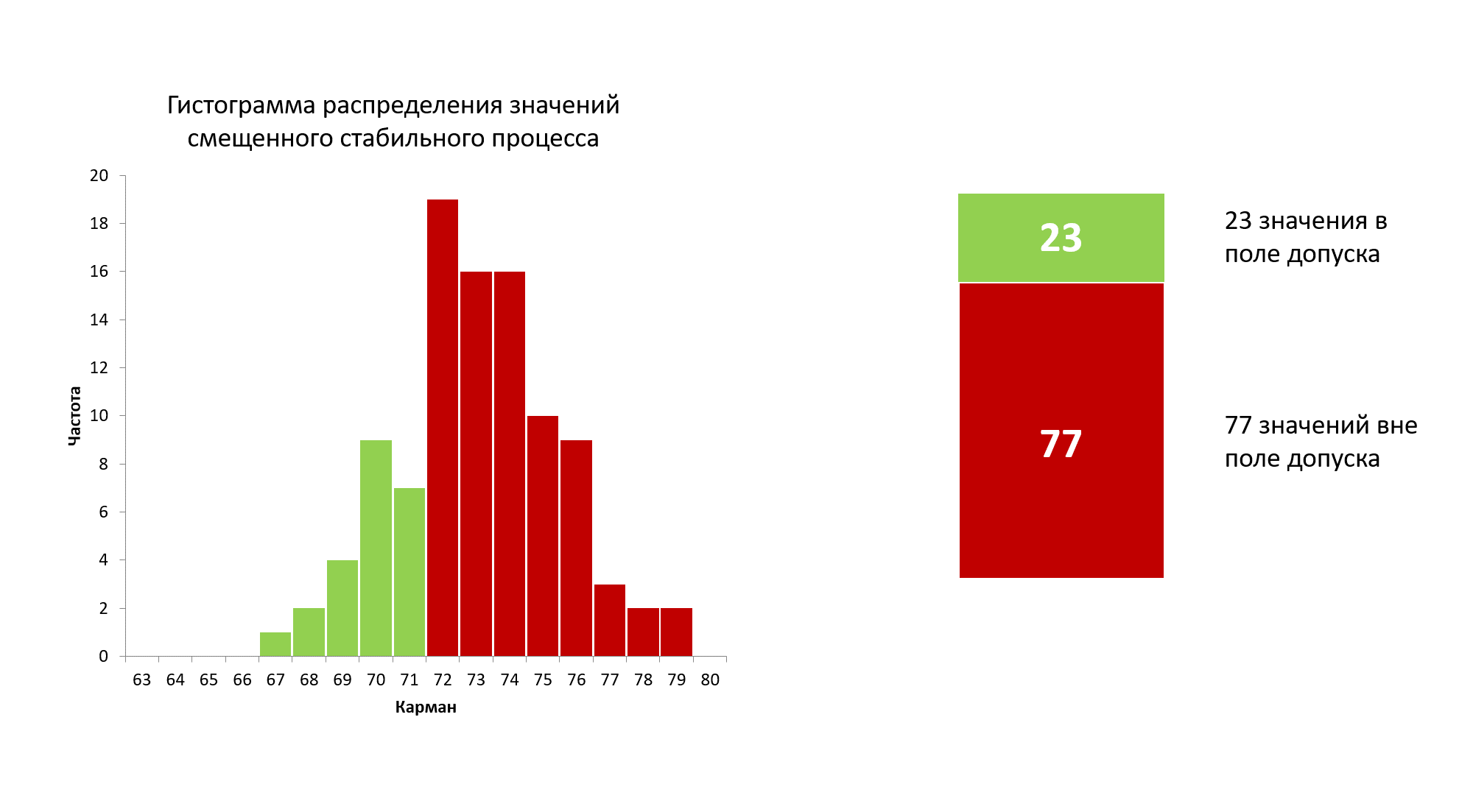
Figure 17: Histogram of the distribution of 100 initial values of a stable but poorly centered process.
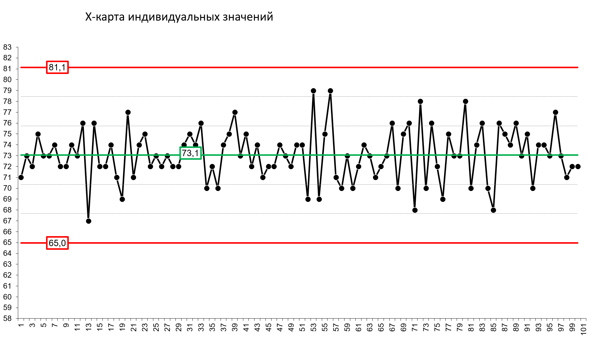
Figure 18. X-map of individual values (process voice) of 100 initial values of a stable but poorly centered process. The red lines, respectively, are the upper and lower natural boundaries of the process, the green line is the central line (average) of the process.
In this case, only one adjustment will be required to center the process within the tolerance range. Simply change the machine setting once to offset the average stable process from the center of the tolerance zone.
So, if the average of a stable and poorly centered process is 73.1, and the center of the tolerance field is 69. The displacement of a stable, poorly centered process: 69.0-73.1 = -4.1
It is by the amount of displacement that the settings of the machine that produces these parts must be changed. And call the technical service, which should set up the machine. See the result below.
Figure 19: Histogram of the distribution of 100 new values after centering in the tolerance field of a stable process.
Figure 20. X-map of individual values (process voice) 100 new values after centering in the stable process tolerance field. The red lines, respectively, are the upper and lower natural boundaries of the process, the green line is the central line (average) of the process. The drawing was prepared using our developed “Shewhart control charts PRO-Analyst +AI (for Windows, Mac, Linux)” .
If you think that the latter case is a rare occurrence, you are very mistaken. If you don't keep control charts of your processes and build histograms of the distribution of indicators relative to tolerance fields, you can't even judge this. If you are familiar with the process performance (reproducibility) indices Cp (living space index) and Cpk (process centering index), then you should know that Cpk in the vast majority of cases is less than Cp, which indicates a shift of the average process from the center of the tolerance field towards the bottom or upper tolerance limit. In any case, centering both stable and any unstable processes in the tolerance zone reduces the share of defective process parts that go beyond the tolerance limits in “one click.” In cases where the process operates within the tolerance zone, centering significantly improves the quality of parts and assemblies (DSE), bringing most of the parts closer to the center of the tolerance zone (for symmetrical tolerance zones). The last statement explains Taguchi loss function .
Process improvements from 77 defective parts to 32 with one adjustment.
“How do you like that, Elon Musk?”
Important!
- The only economically feasible way to significantly improve quality is to first bring the process into a statistically controlled state, and only after that start centering it in the tolerance zone.
- Before any process research, ensure that your measurement system , which is used by the operator making adjustments to the technological process, is in a statistically controlled state, does not have a significant bias, find out whether its accuracy is sufficient for assessing the process, whether the uniform measurements are adequate (measurement depth) or, conversely, whether you are recording noise. - See description of our software Shewhart control charts .
"There is no substitute for knowledge. But the prospect of using knowledge is scary."