The all-or-nothing plan is against the use of tables for random quality acceptance inspection. Edwards Deming
“The use of acceptance sampling inspection tables cannot be adapted to minimize the average total cost of incoming materials inspection and the consequences of allowing defective materials into production.”
Source of cited materials: [2] - W. Edwards Deming, “Out of the Crisis” (“Out of the Crisis”, W. Edwards Deming - M.: Alpina Publisher, 2017. Scientific editors Y. Rubanik, Y. Adler, V. Shper). You can purchase the book from the publisher Alpina Publisher .
The article was prepared by the scientific director of the AQT Center Sergey P. Grigoryev
Free access to articles does not in any way diminish the value of the materials contained in them.
Preface
Should we try to reject some or all of the defective items in an incoming shipment? Or should we send every batch, bypassing inspection, straight into production? An economically sound solution would be to use the “all or nothing” control plan for incoming raw materials, materials and components proposed by Edwards Deming.
In any case, not a single product produced by the company that does not meet the requirements should reach our buyer.
The all-or-nothing input control rule is used to minimize a company's average total cost per unit of production. The “all or nothing” rule is a rule for making a decision about 100% control of an incoming batch of materials with the rejection of defective ones or the release of such a batch into production without incoming control, followed by the replacement and reworking of the proportion of defective products formed as a result of such a pass without incoming control.
If you carry out incoming inspection of raw materials, materials and components for sampling control, it is better to know that:
“If the degree of statistical control over the quality of incoming materials is high, the control of samples would not provide insight into the remainder of the inspected lot, due to the lack of evidence of correlation between them in this case.”
A practical confirmation of Edwards Deming's statement that sampling control, for example, using tables of random acceptance quality control does not give an idea of the number of defective products in the controlled batch, can be experiment with red beads , in which random mechanical samples from a mixture of red and white beads each time give a value for the proportion of red beads that differs from the real proportion of red beads in the controlled mixture, both higher and lower. The experiment used a control np-chart of the number of red beads for samples of the same size.
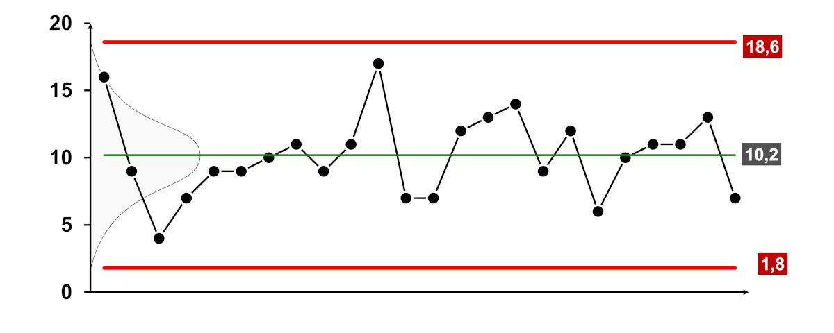
Rice. Control np-chart of the red bead experiment conducted by Edwards Deming in 1983.
“The rules for minimizing total average costs turn out to be extremely simple under some conditions.
Designations:
p is the average proportion of defective products in the incoming batch of parts;
k 1 - cost of incoming inspection of one part;
k 2 - the cost of dismantling, repairing, reassembling and retesting a unit that failed due to one defective part that entered production.
Condition 1:
The worst incoming lot will have an average defective rate (p) less than (k 1 /k 2 ).
p<k 1 /k 2
In this case: No input control. Reliance must be placed entirely on inspection at the point of testing of the components.
Explanation, Sergey P. Grigoryev:
Derivation of the formula Condition 1, when the total cost of correcting all units with defective parts from the incoming batch (N×p×k 2 ) will be less than the cost of inspecting all 100% of incoming parts (N×k 1 ).
(N) - size of the incoming batch of parts, pcs., with the share of defective ones (p):
N×p×k 2 <N×k 1
reduce the expression to:
p×k 2 <k 1
Then:
p<k 1 /k 2
Condition 2:
The best incoming batch will have a proportion of defective items (p) greater than (k 1 /k 2 ).
p>k 1 /k 2
In this case: 100% input control. And carry out control at the point of testing of finished products.
Explanation, Sergey P. Grigoryev:
Derivation of the formula Condition 2, when the total cost of correcting all units with defective parts from the incoming batch (N×p×k 2 ) will be greater than the cost of inspecting all 100% of incoming parts (N×k 1 ).
(N) - size of the incoming batch of parts, pcs., with the share of defective ones (p):
N×p×k 2 >N×k 1
reduce the expression to:
p×k 2 >k 1
Then:
p>k 1 /k 2
(k 1 /k 2 ) - equilibrium quality, or equilibrium point.
(k 2 ) will always be greater (k 1 );
therefore, the ratio (k 1 /k 2 ) will lie between 0 and 1.
If you apply the Condition 2 rule in a situation where the Condition 1 rule should be applied, then the total cost will be maximum. The reverse is also true."
Example (Sergey P. Grigoryev)
Given:
p (average proportion of defective items in the incoming batch of parts) = 0.05;
k 1 (cost of incoming inspection of one part) = 100.00 ₽;
k 2 (the cost of dismantling, repairing, reassembling and retesting a unit that failed due to one defective part that went into production) = 1,000.00 ₽;
input lot = 1,000.00 pcs.
Condition 1: p<k 1 /k 2 - No entry control.
Condition 2: p>k 1 /k 2 - 100% incoming control.
Calculations
p = 0.05
k 1 /k 2 = 100.00 ₽ / 1,000.00 ₽ = 0.10
0.05 < 0.10
p<k 1 /k 2 - corresponds to Condition 1 - No input control.
Solution
Select the “No control” plan.
Checking the solution
The cost of 100% control at the entrance will be:
1,000 pcs.×100.00 ₽=100,000.00 ₽
The cost of passing defective materials will be:
1,000 pcs.×0.05×1000.00 RUR=50,000.00 RUR
Consequently, allowing a defective part into production, in this case, with subsequent dismantling, repair, reassembly and testing of a unit that failed due to one defective part entering production, will indeed cost 50,000.00 less than 100% incoming inspection ₽.
"Thus, a state of statistical control has a clear advantage. To know whether the incoming batch flow meets Condition 1 or Condition 2 or is in a state bordering on chaos, one only needs to track statistical control and the average defective rate using charts built on the basis of ongoing small sample trials (as in any case), preferably in collaboration with and on the supplier's premises."
Other conditions observed in practice (Edwards Deming)
An intermediate position of the distribution with a moderate deviation from statistical controllability.
We will now analyze two types of intermediate situations for the distribution of the proportion of defective items in incoming lots. Perhaps, using our own control charts, or the supplier's charts, or charts maintained jointly, we can predict that only a small part of the distribution will fall to the right of the equilibrium point. For this case we can adopt a “no control” rule. This rule will allow us to approach the minimum of average total costs, provided that the part of the distribution that lies to the right of the equilibrium point is small.
The opposite situation: only a small part of the distribution of the share of defective products in incoming batches lies to the left of the equilibrium point. Knowing this, you can safely accept the rule of 100% control of incoming batches.
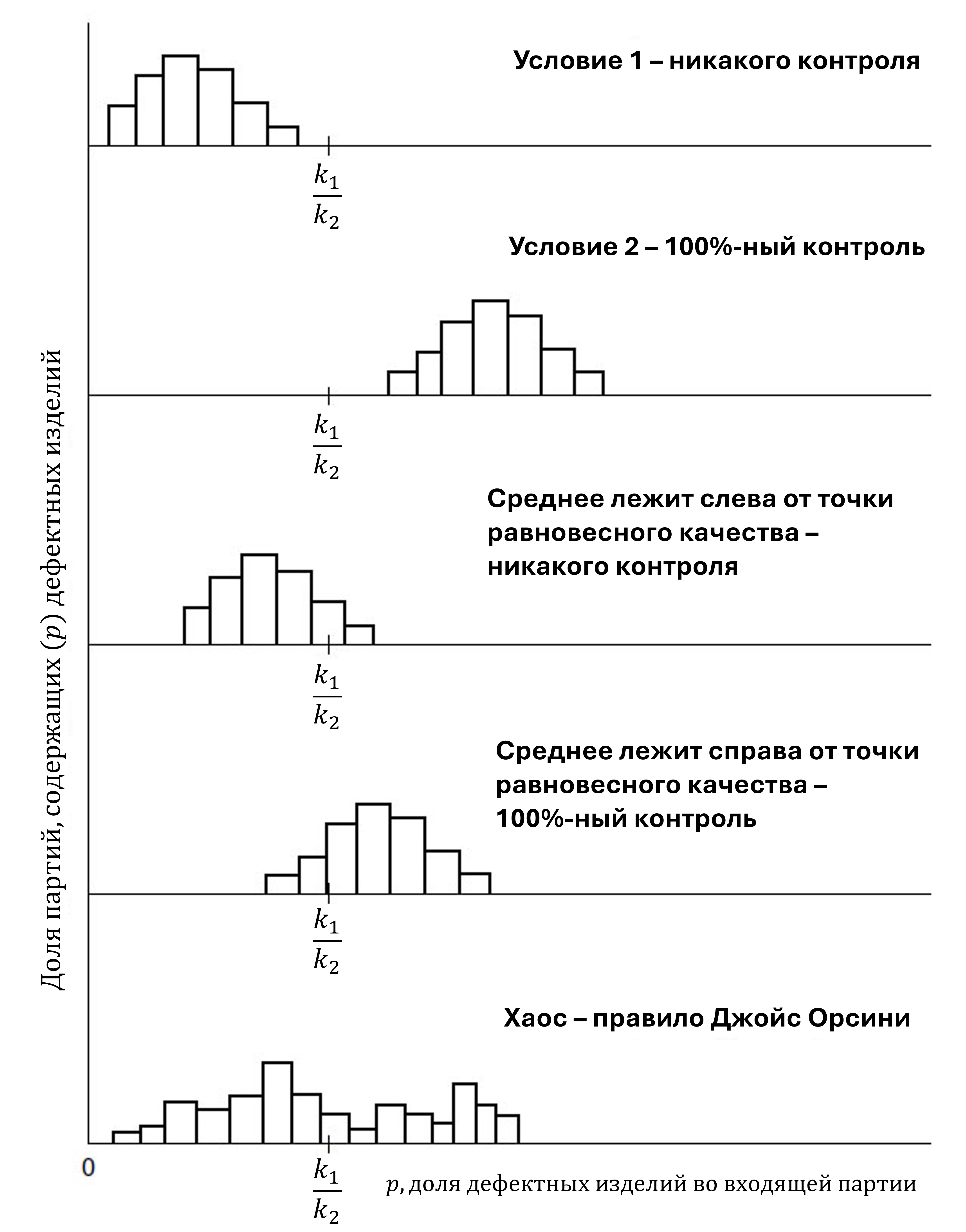
Rice. 1. Possible situations when receiving incoming products in batches.
Point B is the point of equilibrium quality, at which p = k
1
/k
2
. Source:
[2]
Edwards Deming, Out of the Crisis
Trend in the share of defective products in incoming batches
Let us assume that a trend has formed towards an increase in the proportion of defective products. Today we are in Condition 1 and have no control, but (p) is time dependent and increasing, perhaps at a constant rate and perhaps irregularly. In two days we will enter the Condition 2 zone: we have been warned. The supplier's control charts or ours will reveal a trend if one exists. This problem can be easily solved.
Problems caused by switching between different suppliers
Due to changes in material sources at the input of the system, problems always arise. Let us limit ourselves to considering two sources. If both sources are well or moderately statistically controlled and can be separated from each other, then in principle each source satisfies Condition 1 or Condition 2, depending on whether the mean of that source falls to the left or to the right of the equilibrium point. This idea is simple in words, but may prove difficult to implement in some plants.
If materials from two sources are mixed homogeneously in constant proportion, and if both sources exhibit sufficient statistical control, then the mixed batches can be considered as a binomial mixture, the minimum average control cost of which can be achieved using the all-or-none rule.
Materials from two sources bring additional problems to production. A homogeneous mixture of materials from two sources is the worst case scenario for a manufacturing manager.
The first step is to reduce the number of suppliers to one. If a product of variable quality is supplied by a single source, then the supplier and its customer must work together to improve it, aiming to meet Condition 1 and ultimately achieve zero defects.
State of chaos
Deciding what to do in a situation where the position of the distribution fluctuates slightly closer or further from the equilibrium point is relatively easy.
Near the equilibrium point, it doesn't really matter whether we have 100% control or no control at all. I would choose 100% control to gather information as quickly as possible. If we cannot assert that the quality of incoming materials is predominantly to the right or left of the equilibrium point, but, on the contrary, fluctuates widely, passing through the equilibrium quality point, then we are in a state of chaos.
1. This unacceptable situation may arise when material with high variability and unpredictable quality is supplied from a single source.
2. Such variation around the equilibrium quality point may result from obtaining material from two or more sources of widely varying quality. In this case, switching from one source to another is carried out uncontrollably, without a thought-out sequence. We should get out of this state as quickly as possible and move to Condition 1. But the batches keep coming, and we have to do something with them. How should we deal with them?
If each batch came with a label telling us the proportion of defective items in it, there would be no problem. We would achieve minimum average total cost by placing each batch, one after the other, to the right or left of the equilibrium point and applying the all-or-nothing rule from batch to batch.
But the batches are not marked. However, in a state of chaos there is some correlation between the quality of the products in the sample and the rest of the batch. Therefore, in a state of chaos, you can test samples and, using some rule, decide whether to send the remaining part into production completely or to reject it.
Sampling, no matter how well it is used, will result in some lots ending up on the wrong side of the equilibrium point, with the consequence of maximizing total costs for the misidentified lot.
In a state of chaos, one might be inclined toward 100% control. This decision makes some sense.
Never be left without information
The rule of no entry control does not mean driving in the dark with the headlights off. All incoming materials should be reviewed (possibly skipping some lots) to obtain information and compare the actual delivery with the supplier's shipping notes, inspection of the supplier's tests and the accompanying control charts. If there are two suppliers, keep records for each separately.
The next piece of advice is to go to one supplier for each product based on a long-term relationship and work with them to improve the incoming quality.
Destructive testing
The previous theory is based on non-destructive testing of a prototype. Some tests are destructive; they destroy the controlled sample. An example is the life of a light bulb, the number of thermal calories produced by burning a cubic foot of gas, or the operating time of a fuse, or testing the wool content of a piece of cloth. Rejecting the entire batch would not make sense, since there would be nothing to transfer to production.
Obviously, for destructive testing, the only solution is to achieve a state of statistical control in the production of parts in order to immediately make them correctly. This solution is the best for both destructive and non-destructive testing.
Possibility of defective assembly of many parts
In the previous sections we talked about simple products consisting of one part. Some parts may require 100% inspection to minimize overall cost. Once tested, they will not cause the assembly (assembly) to fail. The remaining parts will not be tested, and the defective part, if it enters production, will cause a failure. Let's say we have two untested parts.
Two untested parts have shares of defective p 1 and p 1 . Then the probability that the assembly will fail will be equal to:
Pr (will refuse) = 1 – Pr (won't refuse) = 1 – (1 – p 1 )(1 – p 2 ) = p 1 +p 2 -p 1 p 2
If both p values 1 and p 2 -small, then this probability will be close to the value:
Pr (will refuse) = p 1 +p 2
A simple way to write the probability of failure for any number of parts is to use Venn diagrams (described in any book on probability theory).
Provided that all p i small. Generalization to m parts gives:
Pr (will refuse) = p 1 +p 2 + … + p m
Thus, the probability of failure increases as the number of parts increases. A radio may have 300 parts, although this number will depend on how you count them. A car can have 10,000 parts, again depending on how you count. Is the radio in a car one part or 300? Is the fuel pump 1 part or 7? No matter what you think, the number of parts in a single assembly can be overwhelming.
` But there is another problem: k 2 (the cost of correcting a defective assembly) increases as the number of parts increases. When an assembly fails, which part is at fault? It's all too easy to misdiagnose. Moreover, of two parts, both may be defective.
For products consisting of many parts:
1. We can allow only a few parts to meet Condition 2 (100% control); otherwise the cost of control will be excessive.
2. For other parts, only quality close to zero defects is acceptable.
Assemblies from complex components
Possible savings when creating auxiliary subsystems. In the previous theory, the cost k 2 typically increases (possibly a 10-fold increase) with each step of the process and can reach very high values during final assembly. Sometimes unnecessarily high costs can be avoided by creating subsystems that move along the flow assembled and form the final product. Some subsystems, having passed through control and requiring minor replacements and adjustments, form a new starting point. Cost k 2 will now be the cost of monitoring and adjusting the subsystem. Theory, coupled with useful records of experience, can show that some subsystems do not need to be tested at all, while others should be subject to 100% control to avoid cost increases as the process progresses. The theory presented in this chapter allows you to make the right decision.
Our goal in the preceding sections is to show that there are ways to minimize costs and maximize profits if you follow the right theory.
At the same time, we make every effort to completely eliminate defective products from the process. We do this systematically by comparing our test results with those of the supplier and applying suitable statistical methods such as X- and R-charts (Shewhart control charts).
Fruitful cooperation with the supplier of parts, especially critical ones, and successful testing and adjustment of subsystems reduce all major problems during the final inspection of systems to rare events.
Incoming material is a by-product for the supplier
When a customer-critical material for a supplier may be a by-product, representing less than 1% of its business. The supplier cannot be expected to bear the cost and risk of installing equipment to improve the product.
A possible recommendation is to consider this material as iron ore or other inputs that are highly variable and not purified. Install your own material cleaning system or use the services of a third party company. This plan is effective in some cases.
Difficulties in detecting rare defects
Rare defects are difficult to detect. As the proportion of defective products decreases, it becomes increasingly difficult to determine how small the number is. It is not possible to detect all defects using inspection, especially when they are rare, and this is true for both visual and automatic inspection. There is no reason to trust a manufacturer who claims to have only 1 defect in 10,000 any more than one who claims 1 defect in 5,000 products. In both cases, this proportion is difficult to estimate.
Thus, if (p) were equal to 1/5000 and if the process were in a statistically controlled state, then 80,000 parts would have to be inspected to find 16 defective ones.
Sergey P. Grigoryev:
5000×16=80000
These data would give an estimate of the average defective rate of p = 1/5000 for a production process with a standard error of σ = √16 = 4. This estimate of the defective rate is imprecise, despite the difficulty of monitoring a lot of 80,000 parts. The question arises: did the process remain stable throughout the production of 80,000 parts? If not, what is the meaning of the number 16 defective products? Difficult question.
Sergey P. Grigoryev:
In this case, if the supplier’s process is in a statistically controlled state, it is assumed to operate around the average value c = 16 defects for batches in the form of subgroups of 80,000 parts in size with the values of the upper (VKG, UCL) and lower (NKG, LCL) control limits C- charts: UCL, LCL = c ±3σ or UCL, LCL = c ±3√c, which results in a spread of values around the average (c=16) within ±12.
The formulas can be found in GOST R ISO 7870-1-2011 (ISO 7870-1:2007), GOST R ISO 7870-2-2015 (ISO 7870-2:2013) - Statistical methods. Shewhart control charts [eleven] .
To calculate (σ), Deming uses a C-chart of the number of defects per constant definition area equal to 80,000 parts.
Why 16? The average value (16) allows easy calculation of the (σ) value for the C-chart and provides lower and upper control limits.
Thus, for a supplier to claim such a defect rate (1/5000) requires an understanding of the stability of its production process, which can only be confirmed using Shewhart control charts, and the control chart must be constructed, for example, at a minimum of eight points, where each point is the number of defects per batch of 80,000 parts with possible integer values from 4 to 28 defects distributed over rule of thumb around the average: 16 defects per batch of 80,000 parts.
Why was it impossible to carry out these simple mathematical operations with the average value of defects c = 1 for a constant domain of definition of 5000 parts? Yes, because you will not be able to get points from integers of the number of defects on the control chart below the average value c=1, except zero. Although mathematically it is easy to obtain a decimal number in calculations, for example, = 0.3, how do you imagine the possibility of obtaining in real conditions the number of defects of 0.3 in a tested batch (subgroup)?
There are examples when there is not a single failure in millions of parts, or their number is very small or they are missing in 10 billion. No control of finished products will help obtain the required information when the proportion of defective products is so small. The only possible way to know what is happening at such extreme demands is to use control charts with actual measurements of the parts during the process. One hundred observations, such as 4 items in a row 25 times a day, would yield 25 sample points for X- and R-chart of subgroup means and ranges. Shewhart control charts would show whether the process is proceeding unchanged, or whether a failure has occurred somewhere and the production of a number of products must be stopped until the cause is discovered. Once the reason is found, you can decide to reject the entire set of products for a certain period or skip some products. The ever-increasing capabilities of XbarR control charts of average and range subgroups are becoming more and more obvious.
Sergey P. Grigoryev: Donald Wheeler in the article Control charts for alternative data (counts) p-chart, np-chart, C-chart and u-chart or one XmR-chart of individual values? reinforces this recommendation by Edwards Deming:
"Since it rarely makes sense to use discrete quantities (counts) when measurement results can be obtained, the use of attributes is generally limited to situations where "bloopers" can be counted. However, defining a "blooper" usually poses great difficulty. The main difficulty in defining " blooper" is a problem operational definitions ".
Using reservations
Sometimes it is possible and reasonable when designing complex equipment to place two or more parts in parallel, so that if one of them fails, the other will automatically take over its functions. Two parallel parts, each with an average defect rate p i , are equivalent to one with an average defective rate equal to p i ². If, for example, p i =1/1000, then p i ²=1/1000000.
Weight and size restrictions may, of course, prevent the use of redundancy.
There are other concerns: will the backup part work when needed? Perhaps the best solution is high reliability in a single part.
Conclusion
Defective materials and workmanship will not be tolerated in the manufacturing process. The theory outlined above teaches us how important it is not to tolerate defective materials at any stage of production. The product of one operation is the input material for the next. A defective material, once produced, remains defective until the defect is discovered, if luckily, later in testing, however, correction and replacement will not be cheap.
The state of statistical controllability has a clear advantage. To know whether the incoming batch flow meets Condition 1 or Condition 2 or is in a state bordering on chaos, one need only monitor statistical control and the average percentage of defective items using Shewhart control charts constructed from ongoing tests of small samples (as in any case), preferably in cooperation with the supplier and on his territory.
Exceptions
Many input materials do not follow the theory outlined above. For example, a tank of methanol after stirring with an air hose. A methanol sample taken from almost any part of the tank will be almost the same. However, chemical companies sample methanol at several levels. Perhaps a closer example is sampling a shot of gin or whiskey. We agree that it doesn't matter where we take the portion from: from the top, from the middle of the bottle or from the bottom.
Explanation Sergey P. Grigoryev: The paragraph above refers to exceptional cases when the result of sample control can be attributed to the entire batch.
Blast furnace heating creates problems, and is another example to which the theory in this chapter does not apply. Heating is not uniform. Some companies take small samples from each bottling. These samples, if analyzed, provide data for a process chart that could show variations in quality from the first to the last cast, providing clues to improvements.
Explanation by Sergey P. Grigoryev: The paragraph above deals with exceptional cases when the process is, by definition, heterogeneous at different stages of the process with the possibility of taking one sample from each stage; in such cases, to analyze the variation between different batches (castings), it is necessary to use a control XmR -map of individual values.
See open source solution: Problems of using tables for random acceptance quality control .