Statistical process control (SPC) against the erroneous practice of rationing (timing) of production processes and operations. And how Shewhart control charts help improve production planning.
Material prepared by: Scientific Director of the AQT Center Sergey P. Grigoryev .
Free access to articles does not in any way diminish the value of the materials contained in them.
“Quality-based management significantly changes the understanding of the role of the manager. The manager must become a leader whose main task is to create a system that enables employees to work effectively. A necessary condition for the implementation of this role is the leader’s understanding of the differences between general and special causes of variability.”
The universally applied standardization procedure for processes and operations completely ignores the nature of the variability of the work being standardized. Because of this, it doesn’t even make sense to talk about standardizers and managers taking into account the differences in states in which the work being standardized can be found, namely statistically controlled (predictable behavior) or statistically uncontrollable (unpredictable).
Just think about it! You "normalize" by making a point estimate of a process or operation at a random point in time, and then use this data in planning and control.
In a state of complete chaos, rationing helps to gain some insight into a process that you know nothing about, but then acts as a barrier to process improvement. Why bother improving processes if their standardized indicators are met? If they are not observed, we deprive and fine the “guilty switchmen.” If the norm overlaps for the better, we reward those “involved” and, perhaps, revise the “norm” in the direction of tightening it.
Answer the question: If the graph (Fig. 1.) displayed an important output of one of your processes, for example, output per shift, where on the vertical axis you would set a “real” goal (plan, norm, task) for this indicator for the next shifts or shift assignment? In which gray point or zone from 1 to 4? Remember your answer.
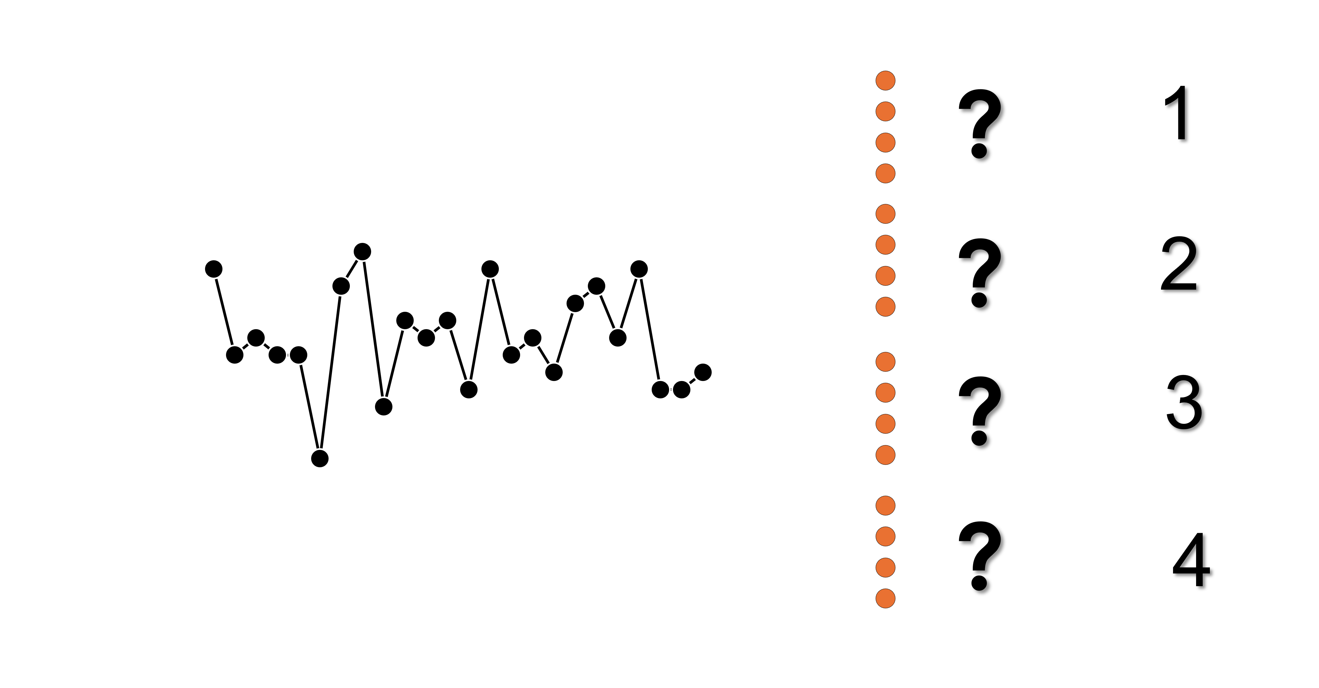
Figure 1. Process timeline. At what gray point will the “real” numerical goal of the process be located?
Evidence 1
The process subject to "normalization" is in a statistically controlled state. If you selected a target in zones 2 or 3:
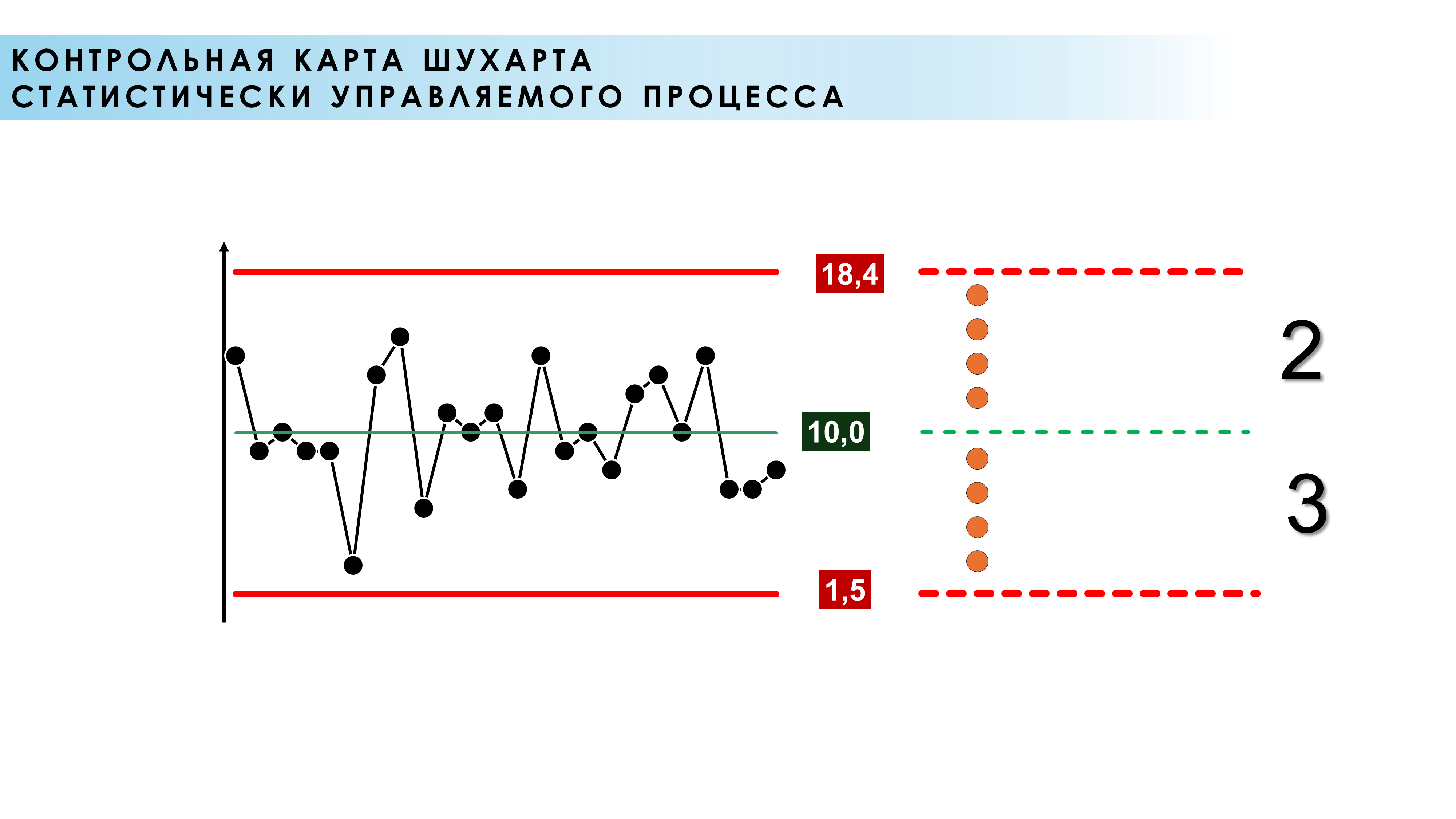
Figure 2. Shewhart control chart for a statistically controlled process. Numerical target for a process in zone 2 or 3. CL - middle line, ВКГ - upper control limit, LKG - lower control limit
Answer: When a process exhibits a reasonable degree of statistical control, the behavior of the process is predictable and it is in its best state. Such a process (and the people in it) does everything it can (see Fig. 2). Knowledge of the past behavior of such a process can be used to predict its future, namely random variations within control limits with the data distributed according to a rule of thumb (Fig. 3). To better understand the material in this article, we recommend that you first read the article: The nature of variability (variations, changeability) is the basis of statistical thinking .
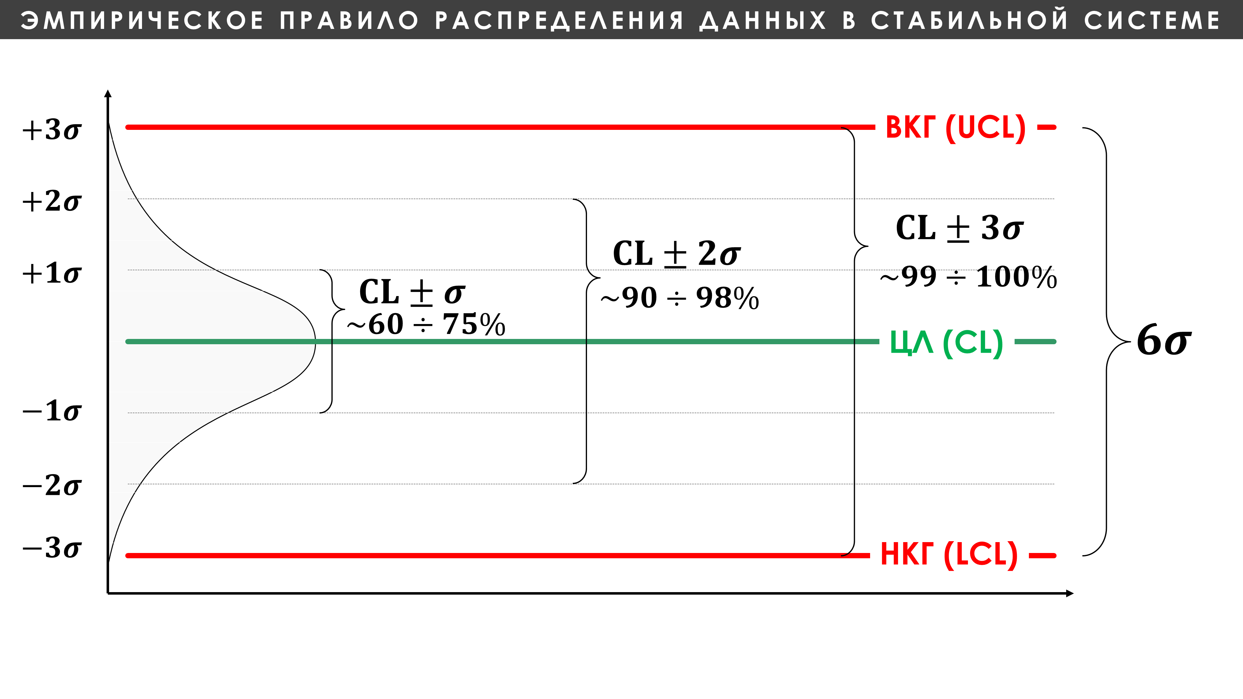
Figure 3. Rule of thumb for data distribution in a stable system. Shewhart control chart. LCG - lower control limit of the process, ВКГ - upper control limit of the process.
"The rule of thumb provides us with a useful way of describing data using a measure of position and a measure of dispersion. If given a homogeneous set of data, then:
1) approximately 60–75% of the data are within one sigma unit on either side of the mean;
2) approximately 90 to 98% of the data lie within two sigma units of the mean;
3) approximately 99–100% of the data are no more than three sigma units away from the average.
The sigma unit (σ) is a measure of the scale of the data. General scattering statistics can be converted to (σ)-units using published formulas*."
* Formulas for calculating σ-units, see [11.1] GOST R 50779.42-99 (ISO 8258-91).

Figure 4. Demonstration of the data distribution and the corresponding control XbarR-chart (XR map) of the means and ranges of subgroups for a process that does not change over time and is in a statistically controlled state (stable process).
Think about it: did the standardizers do their work with a process that was in a statistically controlled state? How do you know? On which day (point)?
In this case (Fig. 2), intervention in the work of the process in the form of specific numerical goals and norms established at any point between the upper and lower control limits along the vertical axis is a “game of roulette” in a limited range. Such a game has nothing to do with planning, much less process improvement.
If you selected a target in zones 1 or 4:
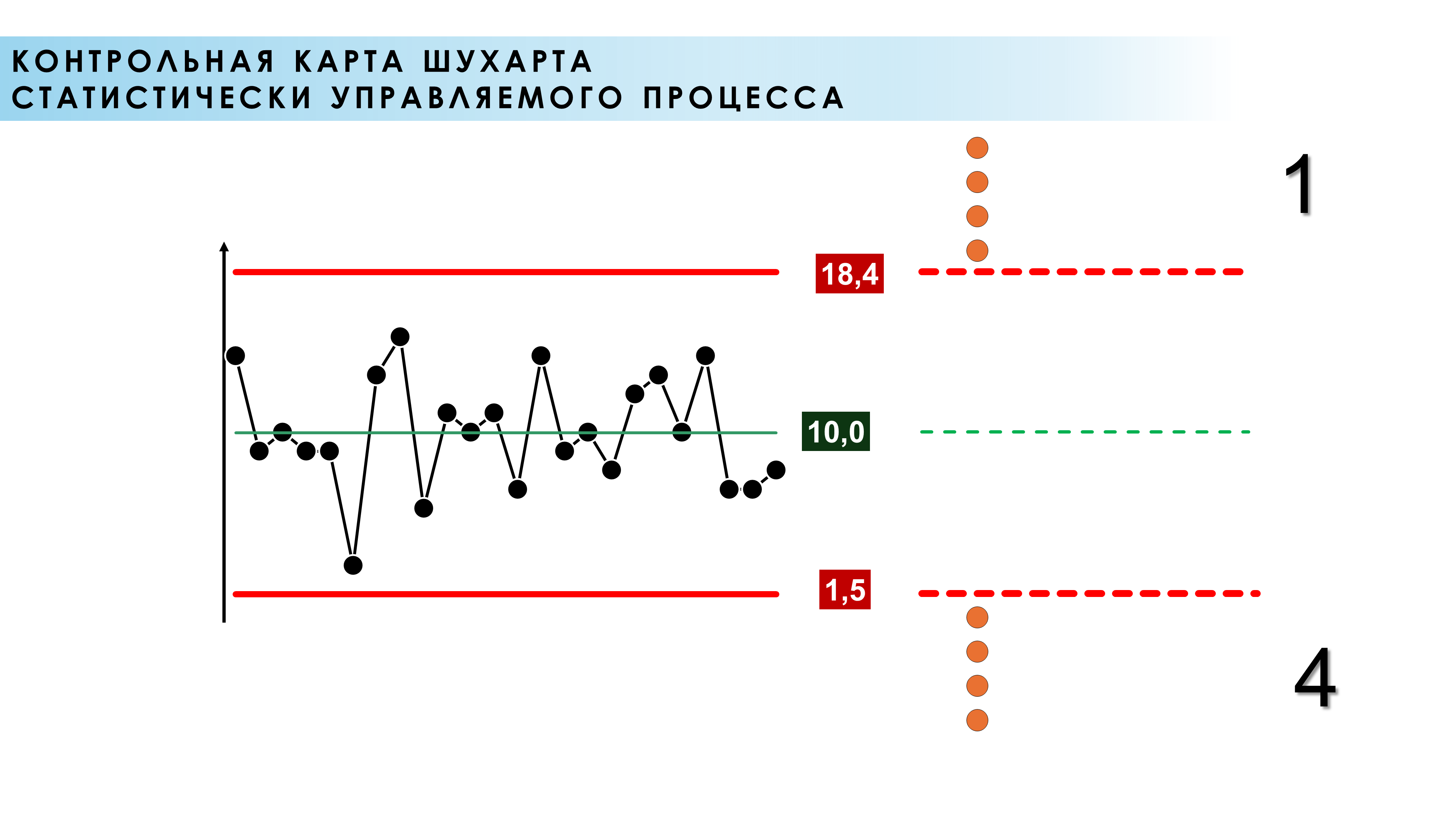
Figure 5. Shewhart control chart for a statistically controlled process. Will the “real” numerical process goal you set be located above the upper or lower natural control limits of the process (outside the control limits)? CL - middle line, ВКГ - upper control limit, LCG - lower control limit
A goal outside the control limit range of a statistically controlled process has no meaning for workers.
If the goal is higher than the capabilities of the system (above the upper control limit), then such a goal causes irritation and dissatisfaction among workers. I will not talk about the option of planning by reasonable management for generation below the lower control limit (zone 4), under the same conditions, as an unlikely situation.
Expecting points above the upper control limit or below the lower one (Fig. 5., zones 1 and 4), for a process in a statistically controlled state, is possible only in three cases [1]:
1. Simple data distortion.
2. Distortion of the system (for example, suboptimization on a selected, for example, Indicator 3, to the detriment of other equally important ones). See Fig.6. (before distortion) and Fig.7. (after distortion).
3. Changing the system (process) by management. This is exactly what the company's management should do. See Fig. 8 and 9.
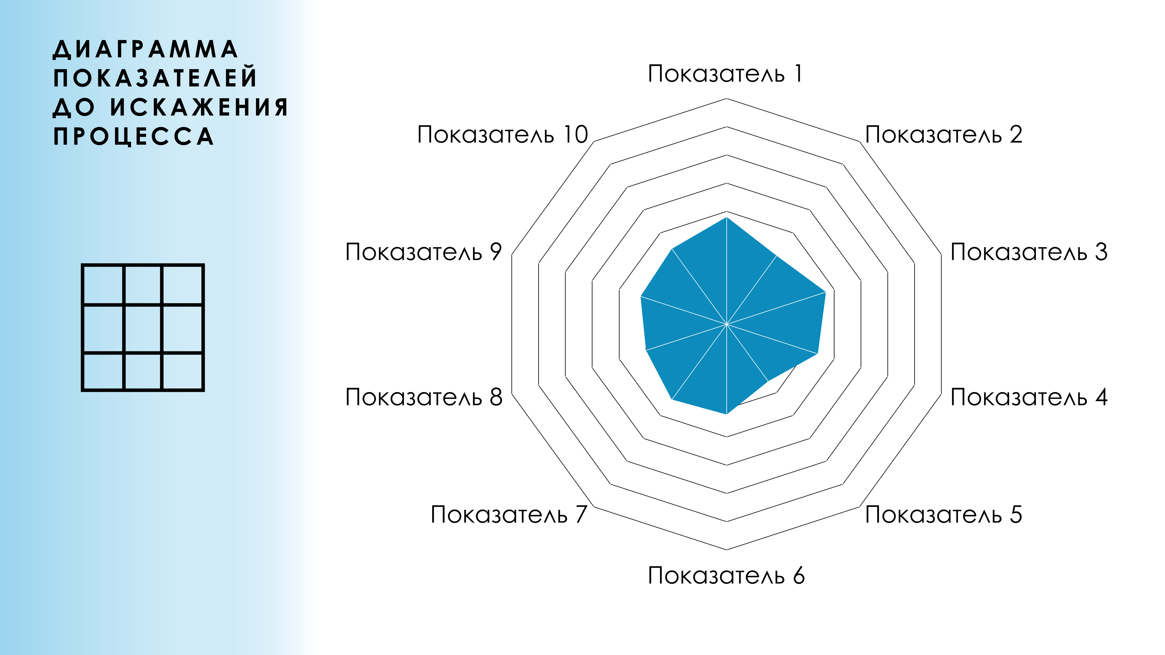
Figure 6. Tracked indicators before the process distortion intervention.
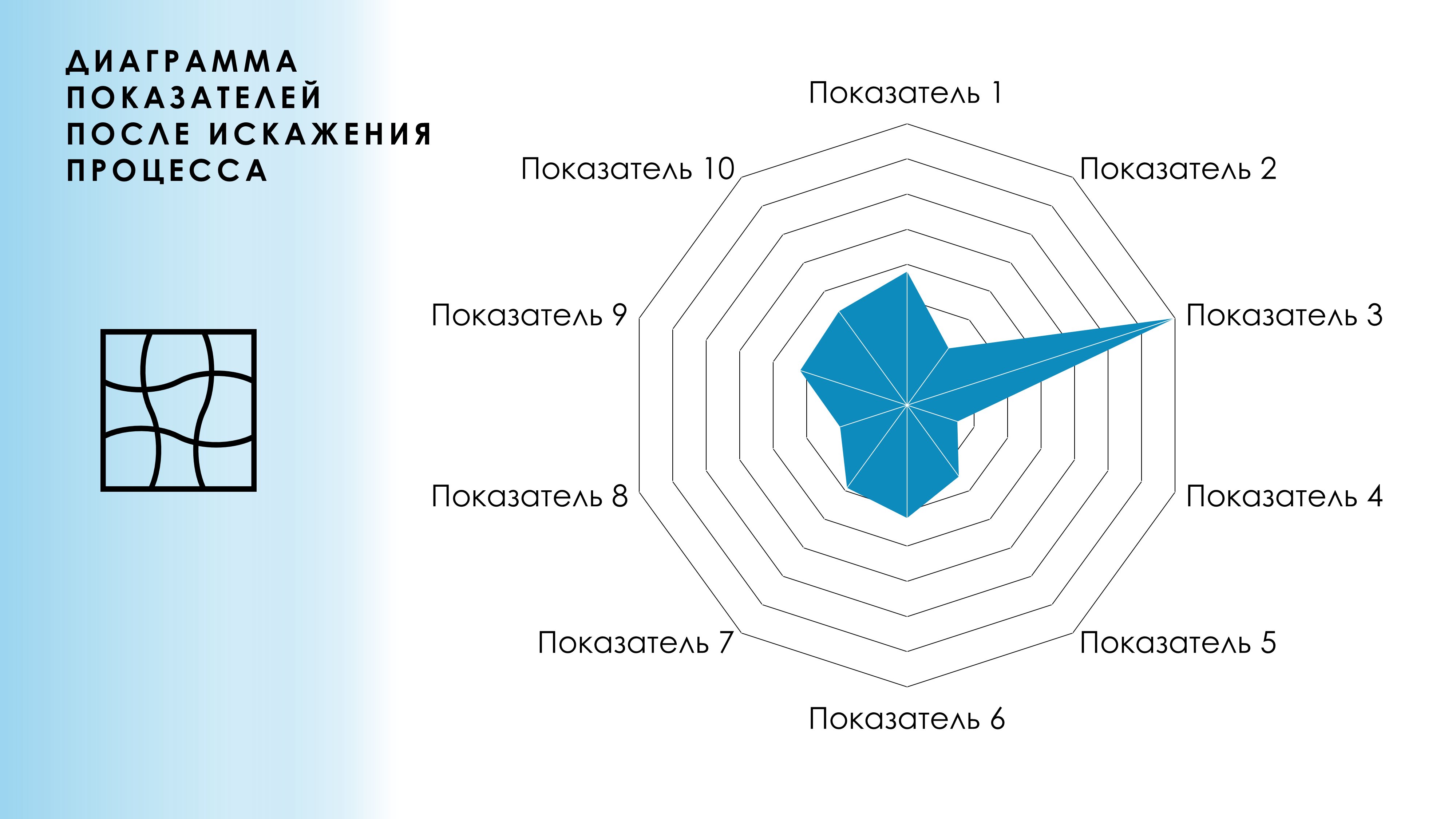
Figure 7. Tracked metrics after process distortion intervention.
The best decision
Searching for specific causes causing observed random variations above and below the mean within a range of control limits, in a process that demonstrates a reasonable degree of statistical control, is not cost effective. For further improvements (shifting the average process towards the desired goal and reducing data scatter), systemic changes are required that are within the competence of top managers, at the level of process design and improvement of all inputs to it, namely: the quality of raw materials and materials, the technical condition of equipment and tools, personnel training, environment, management style, completeness and clarity of technical specifications, etc. Can a worker influence these factors in the result of his activities? A statistically controlled process control chart will always allow you to track the results of any changes undertaken by management. See Figures 8 and 9.

Figure 8. Assessment of process (system) changes in a statistically significant period. Directing the goal towards an above-average process with a constant decrease in variability.
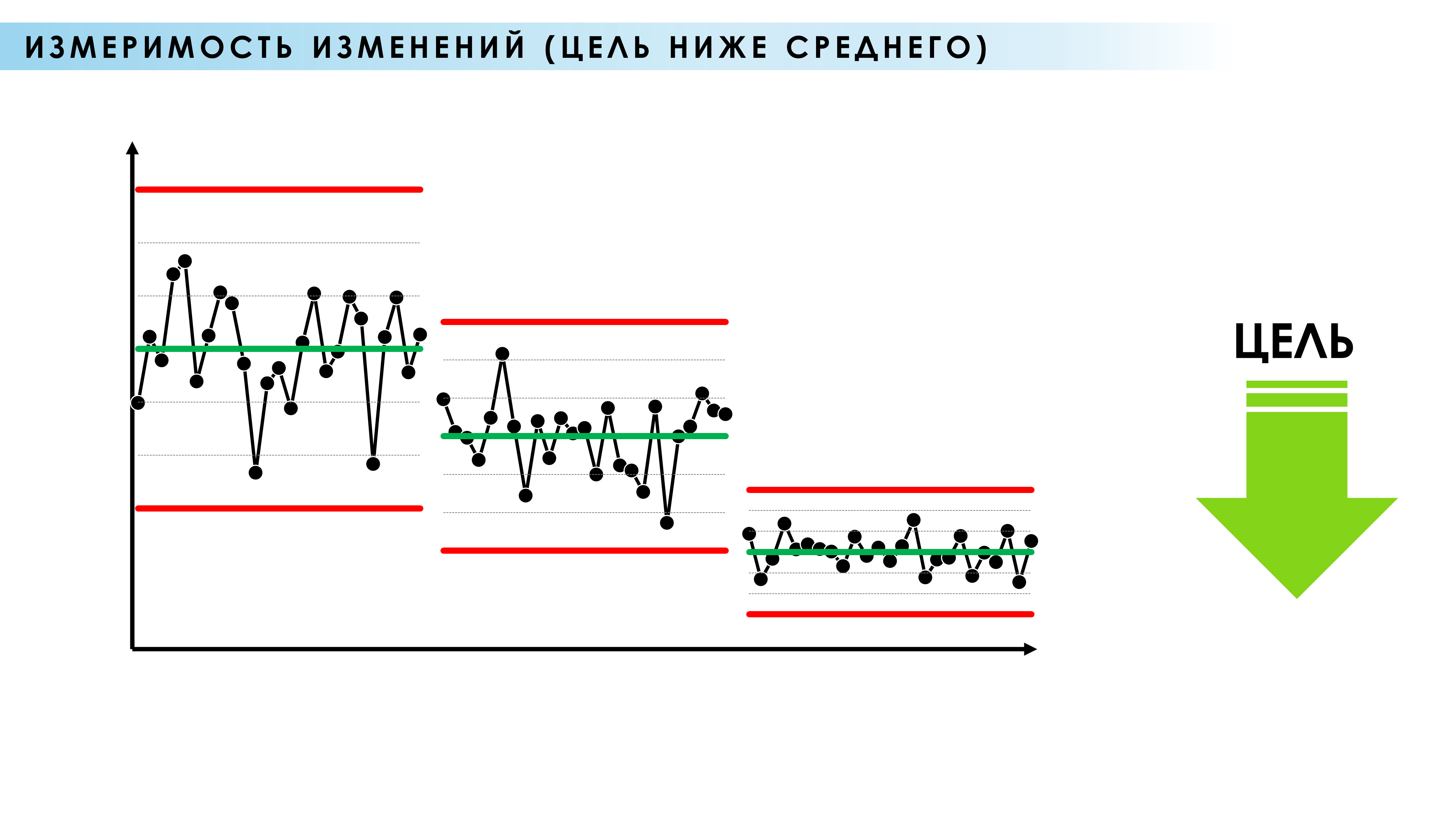
Figure 9. Assessment of process (system) changes in a statistically significant period. Directing the target towards a below-average process with a constant reduction in variability.
Let's go back to rationing
Managers with whom I have spoken always refer to the fact that workers deliberately use “slow” modes when they are “rationed.” Surprisingly, the worker subconsciously feels, although there is no scientific explanation, the influence of chance on his work, more and less than the average. Surely management will accept as normal a random fluctuation of a standardized parameter from the average in the direction desired by management. And the same random fluctuation in the “undesirable” side of the average will be subjected to full analysis and search for special causes. And “those who seek will always find,” even what is not there.
Without enterprise managers understanding the nature of variability, an environment of cooperation between workers and management cannot exist. As a result, distrust of management and fear are maintained. The consequence of workers' fear will be that they will reliably hide problems with processes (information important for process improvement). Is this what you wanted to achieve when you started a program to standardize production operations?
See description of experiments "funnel and target" And "red beads" - Excellent demonstrations of the nature of variation and common management practices.
"No more than 6% of all problems (or opportunities for improvement) in organizations are associated with special causes of variation; thus, they are possibly (but not necessarily!) in the field of activity of ordinary employees. In this case, top managers account for at least 94 % of all potential improvements to the system in which their employees work.
No control and no level of professional skill of workers will be able to overcome the fundamental defects of the system."
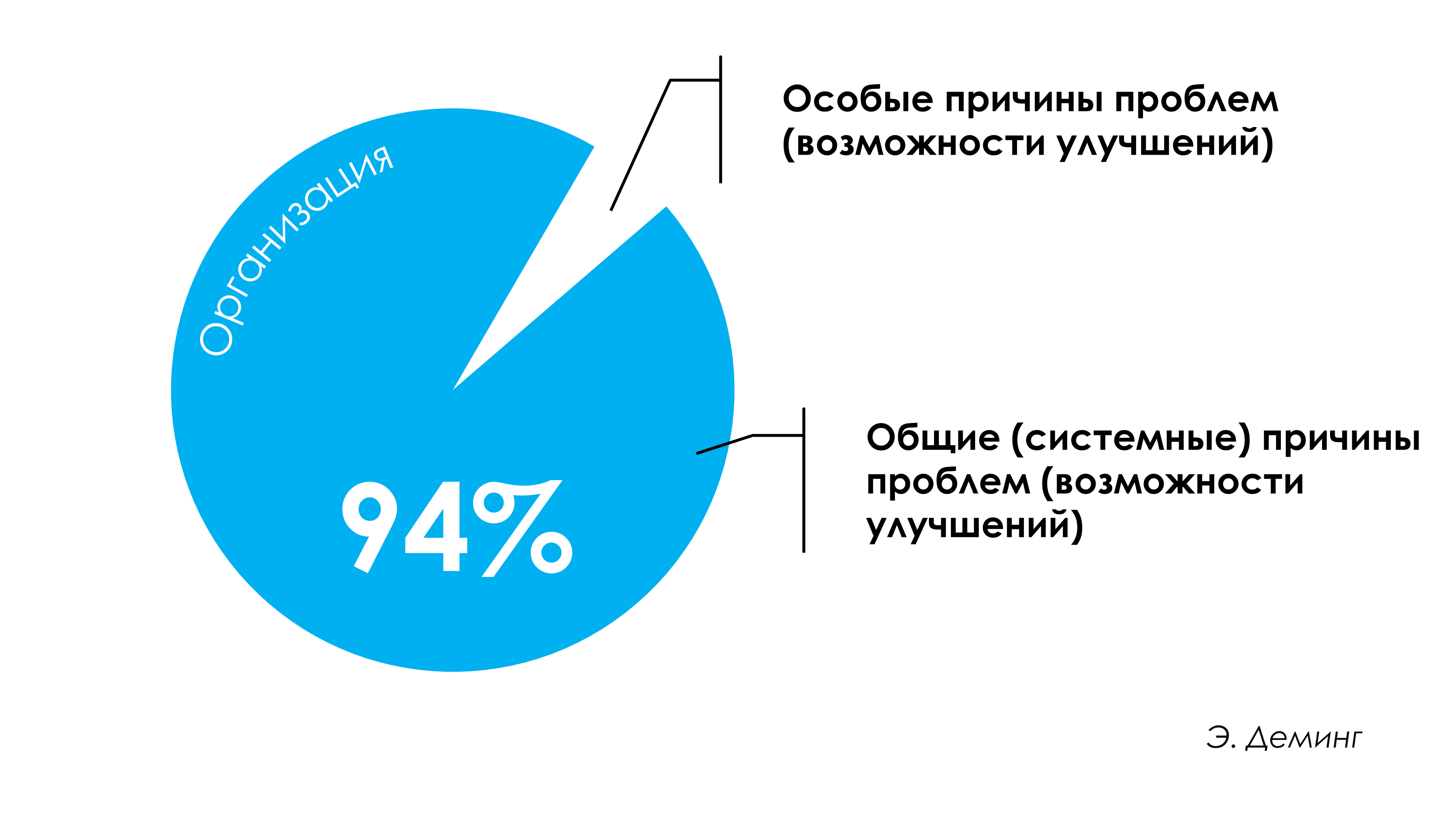
Figure 10. Top managers account for at least 94% of all potential opportunities to improve the system in which their employees work. E. Deming
Evidence 2
The process subject to “normalization” is in a statistically uncontrollable (unpredictable) state.
If a process exhibits a statistically out-of-control state, its behavior is unpredictable (See Control Chart in Figures 11 and 12 below). There is no point in predicting the potential of such a process based on its past and discussing its reproducibility.

Figure 11. Shewhart's control chart for a statistically uncontrollable process and a meaningless numerical goal for it. CL - middle line, ВКГ - upper control limit, LCG - lower control limit.

Figure 12. Demonstration of data distribution and Shewhart control chart of subgroup means and ranges for a time-varying process that is in a statistically uncontrollable state (unstable process).
Think about it: did the standardizers do their work with a process that was in a statistically controlled state? How do you know? Again, on which day (point)?
The total total costs of an uncontrolled process, including those that management does not even take into account, are maximum. To normalize such a process is reckless. First of all, management will need to bring such a process into a state of statistical control, eliminating the special causes of variability, the effect of which manifested itself at the points with the worst results. It will be necessary to find out the specific reasons that caused the points to exceed the control limit with better results, perhaps this is the result of the uniqueness of the employee or his methods, and if these methods are well consistent with the overall goals of the business system, other employees can be trained in them.

Figure 13. The total total costs of an uncontrolled process, including those that management does not even take into account, are maximum.
How then to plan production?
You may object: “Then how can we plan production if there are no standards and a shift plan in the form of a specific number?” You have more than arbitrary norms and assignments when you use Shewhart control charts to study processes. You know what your processes are capable of, and this ability is predictable for processes held in a statistically controlled state. For a hint of a better solution, see paragraph 11. "ELIMINATE ARBITRARY QUANTITATIVE NORMS AND TASKS" Edwards Deming's 14 Points of Management .
For planning, it is necessary to use not “standards pulled out of thin air” or randomly obtained measurement results, but knowledge about the capabilities of stable processes, average and variation in productivity (for example, products per hour). Have an understanding of the rule of thumb for the distribution of data in any system that demonstrates a reasonable degree of statistical controllability (regardless of the shape of the data distribution around the mean), see Figure 3 above.
Of course, this is more difficult than coming up with the desired “number” at the next meeting in the boardroom. You will have to hire a professional in the field of statistical process control, work on studying the properties of your processes, and go down from the offices to the workshop to the workplaces. But this is definitely more effective.
For example, planning orders is carried out according to the average productivity value of the bottleneck (the process with the lowest productivity) in the production chain of processes connected in a line, demonstrating a statistically controlled state.
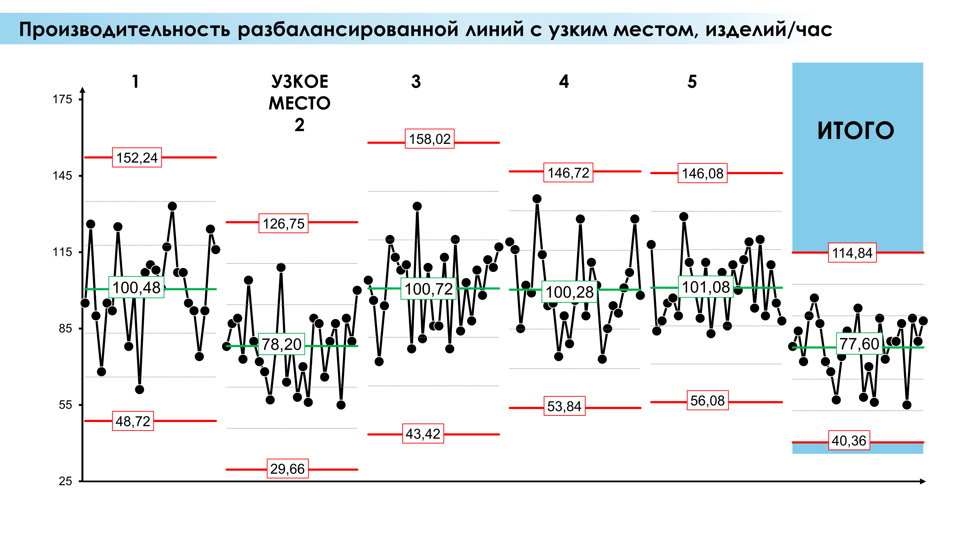
Figure 14. Resulting performance of an unbalanced production line with a bottleneck, demonstrated using Shewhart control charts. The method for analyzing the performance of an unbalanced line, in terms of the simulation method, is borrowed from the book by Donald Wheeler and David Chambers. "Statistical Process Control: Business Optimization Using Shewhart control charts", pp. 366-370 [4]. The drawing was prepared using our developed “Shewhart control charts PRO-Analyst +AI (for Windows, Mac, Linux)” .
The bottleneck in the chain of processes can be easily determined by the presence of the largest interoperational stocks in front of such a process.
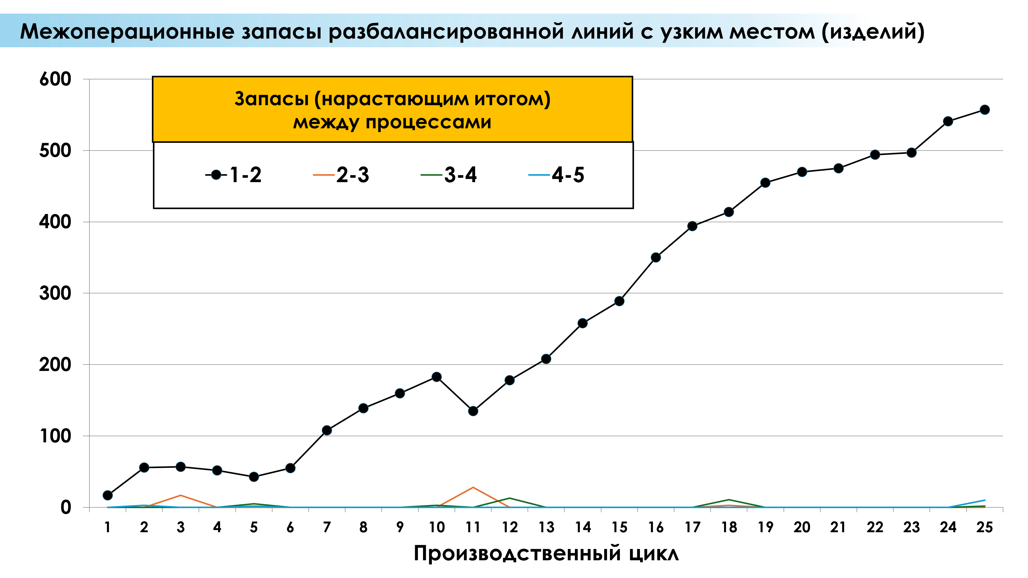
Figure 15. Graph of the build-up of interoperable inventory before the bottleneck in an unbalanced production line with a bottleneck.
It makes sense not to plan volume per shift, but to maintain orders ready to go into production in an “infinite” rolling production plan based on the FIFO principle (a living buffer of orders, some of the first in the queue left, others arrived at the end of the queue). This order buffer is an interoperational stock. Maintain the current buffer volume no lower than the upper performance control limit of the bottleneck in the line, to allow the bottleneck to operate without downtime at random times to achieve its maximum performance. If the process of preparing orders for production is not a bottleneck, this will not require additional effort, since after several cycles such a buffer stock is formed in front of the bottleneck in a natural way.
The control chart will allow you to monitor the state of statistical controllability of processes in the production chain, as well as changes in process performance for the better or worse long before the end of the reporting period. While the processes in the production line are stable, plan the productivity of the line (chain of sequential processes) based on the average productivity of the bottleneck (process) for each type of product.
Do you see any similarities with Goldratt's Theory of Constraints (TOC) developed in the 1980s? Shewhart control charts were developed much earlier and, unlike TOC, take into account predictable or unpredictable process behavior and are based on fundamental science rather than judgment.
Below is an example of the performance of a well-balanced line without bottlenecks. The final performance of a balanced line is always slightly below the average of any process in such a line.

Figure 16. Final performance of a balanced production line without bottlenecks, demonstrated using Shewhart control charts. The analysis method, in terms of the simulation method, is borrowed from the book by Donald Wheeler and David Chambers. "Statistical Process Control: Business Optimization Using Shewhart control charts", pp. 366-370 [4]. The drawing was prepared using the software we developed “Shewhart control charts PRO-Analyst +AI (for Windows, Mac, Linux)” .
Interprocess inventories before the processes of a balanced production line must be maintained at the required level to prevent process downtime. There is no point in accumulating interoperational stock above the upper control limit of the process for which this stock is maintained, for example, when stopping a process in a balanced production line. If all processes operate stably and continuously, in the vast majority of cases the naturally occurring small inter-operational stock will be sufficient for the continuous operation of the entire line (see figure below).
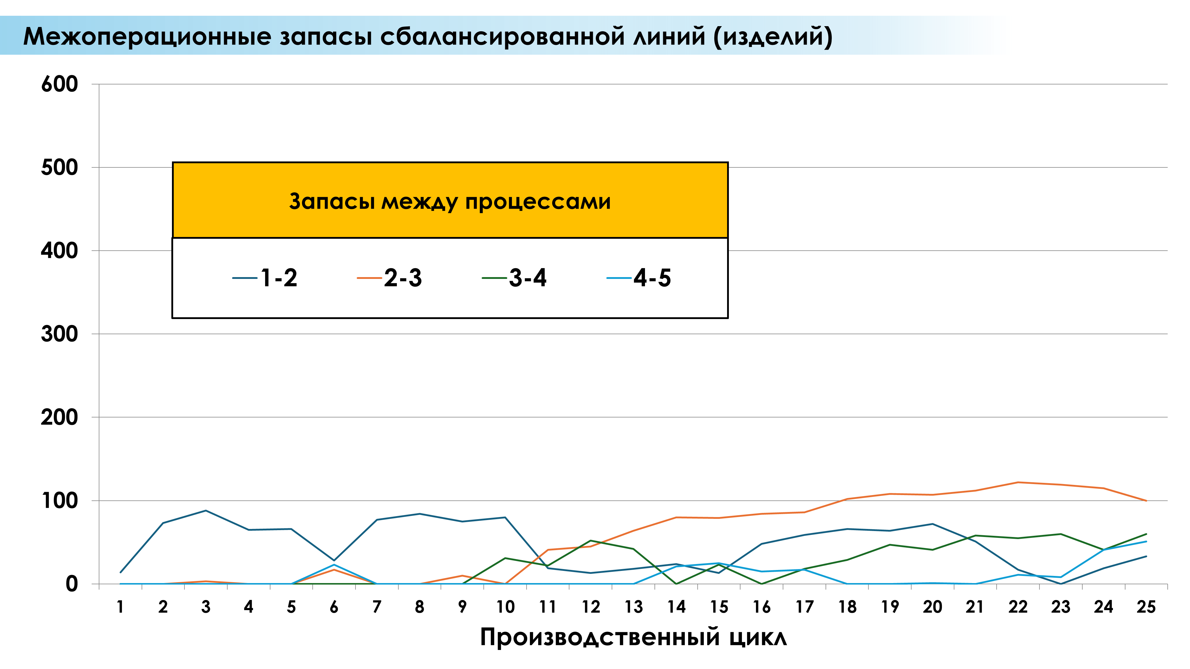
Figure 17. Interoperable inventory accumulation schedule in a balanced production line without bottlenecks.
Constantly improve all processes by reducing the variability of all process inputs (increasing the stability of raw materials, equipment and operations, etc.), introducing innovations. Ishikawa cause-and-effect diagrams, control sheets, Pareto charts, density histograms of individual values, scatter plots, Shewhart control charts are the best tools for this. Moreover, Shewhart control charts are the most important tool. All this will lead to the possibility of more accurate planning. This is a lifelong job and fits well with the goal of optimizing the entire system.

Figure 18. Cause-and-effect diagram. Ishikawa diagram. Fish skeleton.
Did the process improve or worsen (bottleneck)? The control chart will show the change in the mean and range of the data around the mean (easy to see from the range control chart), and the first signs of sustainable changes in the process will be signals indicating a shift in the system. New control limits can be constructed to track the statistical stability of the new state of the process by adding 8 new points of the changed state.
Watch a film about the method of quickly diagnosing changes in a process (system), both positive and negative, using the Shewhart control chart.
Video 1. A method for quickly diagnosing changes in a process (system).
For preliminary calculation of order readiness dates (planning), you can use only process indicators that demonstrate a reasonable degree of statistical controllability (predictability). For example, in serial production for an unbalanced line:
- the average absolute makeready time for each product in its “bottleneck” (absolute value, since in the overwhelming majority, makeready time does not depend on the batch size);
- average productivity per unit of time for each product in its “bottleneck”;
- average of unplanned bottleneck downtime.
From the total daily time corresponding to a specific product of the “bottleneck” of the technological chain, we subtract all planned equipment downtime (maintenance, repairs, non-working hours, etc.).
Control charts of unplanned downtime by type of cause and time in the past will serve two purposes: to work to reduce their number and duration, and for processes (bottleneck equipment) demonstrating a reasonable degree of statistical controllability in terms of unplanned downtime - to take them into account in planning, taking away the average time of such downtime from the working time remaining at the previous step.
For the remaining working time, we distribute orders taking into account the order, average makeready time and average productivity for each type of product. Processes that are in a statistically uncontrollable state are, by definition, unpredictable; their average is unreasonable to use for planning (prediction). To improve the planning system, you will have to bring such processes into a statistically stable (controllable) state, and then work on reducing the variability of such processes.
IMPORTANT
It is important to understand that it is not the planned number (norm) that produces the product, but the processes that do not care about this planned target. We know a lot about processes and people in them if we collect and analyze data and work with people and processes at the shop level (in the gemba). We want to increase productivity - we improve the “inputs” to the process and the process itself through monitoring the “outputs” with an understanding of the matter and using Shewhart control charts for numerically measurable metrics, we optimize the entire system according to its goals.

Figure 19. Functional modeling methodology IDEF0 [16] .